


There are a number of ways in which you can alter the graphical display once you have generated the basic elements in it (contours, meshes, and so on). For example, you can overlay multiple graphics, add descriptive text or lighting to the plot, and modify the captions or legend layout. These and other customizations are described in this section.
- 40.2.1. Embedded Graphics Window Dashboards
- 40.2.2. Advanced Graphics Overlays
- 40.2.3. Managing Multiple Graphics Windows
- 40.2.4. Showing Boundary Markers
- 40.2.5. Changing the Legend Display
- 40.2.6. Adding Text to the Graphics Window
- 40.2.7. Changing the Colormap and Range
- 40.2.8. Adding Lights
- 40.2.9. Modifying the Rendering Options
Important: It is possible that the graphics window may become [Out of Date] (which would be indicated at the top of the graphics window), if you make changes to items that are already displayed. To resolve this out of date state, right-click in the graphics window and click Refresh Display in the context menu that appears.
If a context menu does not appear on a right-click of the graphics window, ensure that the right-mouse button is set to an action other than Zoom or mouse-probe and long description (View ribbon tab, Mouse group box).
For the refresh of a mesh display, Fluent displays the surfaces that
are currently selected in the global Mesh Display dialog box
(accessed by clicking ![]() in the toolbar). In some instances this may result in the
refreshed display not matching what was originally displayed.
in the toolbar). In some instances this may result in the
refreshed display not matching what was originally displayed.
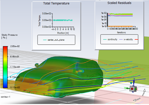
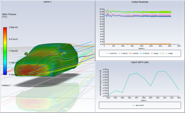
You can embed multiple graphics windows into a separate window (also know as "picture in picture"), like in Figure 40.53: Example of Embedded Windows, which shows residuals and a report plot embedded within the Solution View. The feature lets you create a dashboard-like display containing both 2D and 3D plots, and the Solution View window (see Automatically Embedding Windows in the Solution View) automatically updates the parent window at a set interval, allowing you to see the solution evolve on the displayed quantities. This can be a helpful technique for monitoring solution progress, postprocessing the results, or disseminating your conclusions as a part of a presentation. It is also possible to create an animation of this dashboard, which can then be saved in MP4 and other video formats.
Tip: Display your dashboard(s) prior to beginning your solver run to ensure they appear as desired.
These sections describe the methods for creating embedded window dashboards
Fluent can automatically create an embedded window dashboard for you as soon as you begin calculating a solution. By default (with options enabled in Preferences), the parent window will be a scene graphics object, and the mesh and residuals will be embedded within that parent window (like Figure 40.53: Example of Embedded Windows). If you do not have any graphics objects defined, Fluent will create one for you (3D simulations only).
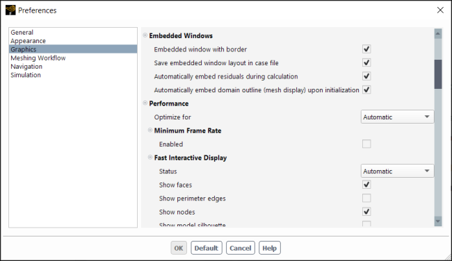
There are two Preferences options for automatically embedding graphics windows: Automatically embed residuals during calculation and Automatically embed domain outline (mesh display) upon initialization. These provide you the choice of what will be done automatically when you initialize the solution and begin calculating. To control these options, open them in Preferences.
![]() File
→ Preferences...
File
→ Preferences...
Automatically embed residuals during calculation—the Residuals graphics window is automatically embedded within the Solution View graphics window as soon as the solver begins calculating. Once embedded, the residuals may be resized and relocated as desired.
You can right-click the embedded residuals windows and select Move Out Embedded Window to make it so the residuals are no longer embedded. To re-embed residuals, right-click the Residuals tab and select Embed In > target-window.
Note: Adjoint residuals are not automatically embedded in the Solution View graphics window. However, you may include them in your embedded window dashboard by right-clicking the Adjoint Residuals tab and selecting Embed In and picking the solution view window as the destination.
Automatically embed domain outline (mesh display) up on initialization—the graphics window containing the global mesh display, that is, mesh either displayed automatically after reading the mesh/case or by clicking the Mesh Display button in the toolbar (
 ), is automatically embedded within the
Solution View graphics window as soon as you
initialize the solution. Once embedded, the mesh may be resized and
relocated as desired. You can also double-click the embedded mesh window
and it will swap with the content displayed in the current parent
window.
), is automatically embedded within the
Solution View graphics window as soon as you
initialize the solution. Once embedded, the mesh may be resized and
relocated as desired. You can also double-click the embedded mesh window
and it will swap with the content displayed in the current parent
window.You can change the contents of the parent window to include any type of graphics display, such as a contour plot or an XY plot. Just right-click the defined object in the Outline View tree and select Display.
Both of the options for automatic embedding create a Solution View graphics window that will contain the parent and embedded windows. Fluent automatically selects the parent window in the following order: scene (Displaying a Scene), contour (Displaying Contours and Profiles), vector (Displaying Vectors), pathline (Displaying Pathlines), particle tracks (Displaying of Trajectories). (3D cases only) If there are not any graphics objects associated with the case file, Fluent automatically creates a plane surface and contour graphics object for the solution view.
Simultaneously with the creation of the solution view window, Fluent creates a temporary Dashboard object that appears in the Outline View tree under Results. This object is deleted if you close the dashboard.
The exact contents of the Solution View window are not saved in the case file, but the layout of the embedded windows is preserved (assuming that Save embedded layout in case file is enabled in Preferences).
Important: Only the object included in the solution-view animation definition is updated at a specified interval while Fluent is calculating. Objects in other windows (for example a mesh plot) embedded on the solution view window are not updated as the solution progresses.
You can create dashboard objects that are added to the tree and stored with the case file using the Dashboard Definition. These dashboards are functionally the same as dashboards created using other means, but their advantage comes from the ability have the dashboard retained with the case file and available in the Outline View tree. Further, these dashboards are easily edited and can be quickly redisplayed.
To create a dashboard using the Dashboard Definition dialog box:
Open the Dashboard Definition dialog box.
 Results
→ Graphics
→ Dashboard...
Results
→ Graphics
→ Dashboard...Enter a Name for the dashboard you are creating.
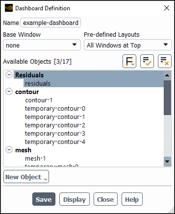
Use the Base Window drop-down list to specify which object will be shown in the large background graphics window that all other graphics objects will be embedded into. Note that you can also leave this option set to none, so that all child windows are embedded into an empty graphics window. This allows you to tile the child windows such that there is no overlap. See Figure 40.55: Dashboard with "none" for Base Window for an example.
Specify where you want the embedded windows to appear when they are first displayed from the Pre-defined Layout drop-down list.
Important:Once the dashboard is displayed, you can drag the embedded windows around as desired. Fluent saves the updated positioning of the windows when you write the case file.
If you change the pre-defined layout after displaying a dashboard, you must close the displayed dashboard and re-display before you will see the updated layout.
Select the windows you want embedded into the Base Window from the Child Windows list.
Click to display the dashboard. Click to save the dashboard with the case file..
Note: If a dashboard is visible in the graphics window, displaying another object (such as a contour or XY Plot) will be displayed in the active dashboard window, which automatically updates the dashboard definition.
Right-clicking an object in the Outline View tree and selecting Display in New Window avoids modifying the dashboard. Similarly, you can right-click the top of the displayed graphics window tab and select New Window to open an empty window for display.
To setup embedded windows:
Ensure graphics objects are available by either initializing the solution or loading a results (data) file.
Create an animation definition containing the desired graphics object(s). Refer to Creating an Animation Definition for additional information.
Note: Embedding into an animation graphics window allows you to see both the 2D plots (such as residuals and report plots) as well as the monitored quantity in the animation definition (whatever is specified within the selected graphics object) updated as the solution progresses.
Additionally, layouts embedded into an animation graphics window are saved with the case and data file and are redisplayed automatically when you begin calculating in another session.
Determine which graphics window you want as the baseline/parent and note its name. You must know the name so that you know which window to select when moving the other window(s).
Important: If you want to save the embedded window layout as an animation, you must use an animation definition as the baseline window. Further, this animation definition must be saved in one of the 2D image formats (that is, PPM, TIFF, PNG, or JPEG). Refer to Creating an Animation Definition for additional information on creating animation definitions.
Once other windows are embedded in the animation definition window, saved animation images will include the additional windows. These animations can then be saved in standard video formats, as described in Saving an Animation Sequence.
Note that the border of embedded windows will not be included in images saved using the Save Picture dialog box (Saving Picture Files) or animations.
Add the windows you want embedded either by:
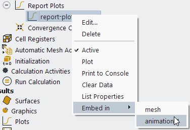
Right-clicking the desired graphics object in the Outline View tree and select Embed in > <target window name> from the context menu. This option is available for all viable object types, including reserved windows such as report plots and animation definitions, even before data is generated by beginning the calculation. See Figure 40.56: Embedding a Window - Outline View Context Menufor an example of this technique.
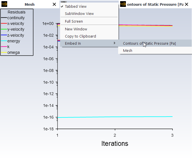
Right-clicking the tab (or top of the window if you are viewing graphics windows as subwindows) of a window you want to embed and select Embed In → <target window name>. See Figure 40.57: Embedding a Window - Tab Context Menu for an example of how this technique. Note that you must begin iterating by starting the calculation, for reserved windows, such as residuals and report plots, to open automatically.
Note: Once you have embedded one window into another, a dashboard-n definition is created and added to the Outline View tree for your embedded window dashboard.
Repeat the previous step for all windows that you want to embed.
Arrange the embedded windows in the best layout for your purposes. You can resize embedded windows by dragging at the edges of the window. You can move embedded windows (within the borders of the baseline window) by left-clicking and dragging at the top of the window.
Save your case and data to save the layout and contents of your embedded window dashboard.
File
→ Write → Case
& Data...The next time you open your case and data, display the baseline/parent window and Fluent will automatically embed the child windows when you begin calculating. Alternatively, you can right-click dashboard-n in the Outline View tree and click Display to display the embedded windows dashboard.
Embedded window dashboards can be animated, allowing you to playback whatever it is that you choose to include in your dashboard. This could include monitors such as report definitions and residuals for checking convergence, or it could be assorted graphics objects focusing on different areas of your model, showing how quantities evolve as the solution progresses.
There are two approaches you can take to create your dashboard animation:
You create your dashboard manually as described in Manually Embedding Windows.
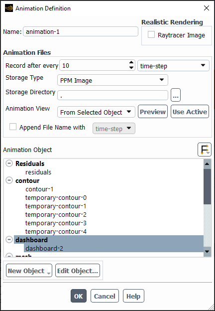
Then you select the defined dashboard as the animation object in the Animation Definition dialog box (see Figure 40.58: Selecting a Dashboard to Animate for an example). Preview the dashboard prior to closing the dialog box, so you can ensure the layout is as desired.
Note that the border of embedded windows will not be included in images saved using the Save Picture dialog box (Saving Picture Files) or animations.
Important: Before beginning the computation, close all windows associated with the dashboard you are animating (that includes any of the objects contained in the dashboard, and the dashboard itself). Click Preview in the Animation Definition dialog box and adjust the dashboard layout as desired, then start calculating. This ensures the resulting animation appears as expected.
Note: When defining the dashboard you want to animate, only include one type of graphics object (contours, vectors, and so on) as the embedded window, or the dashboard may not behave as expected. You can include as many plots (report plots and residuals) as desired.
Fluent automatically generates your dashboard, at least initially, as described in Automatically Embedding Windows in the Solution View. With the Solution View window created, you can control which object is represented as the parent window:
Make Solution View the active graphics window by clicking the tab or sub-window.
Click inside the parent window to make it active. This ensures that the graphics object that you display in the next step replaces the current parent window, rather than replacing one of the embedded windows.
Right-click the desired graphics object in the Outline View tree and select Display in the context menu that appears.
Specify how frequently you want the parent dashboard window to be updated and whether or not you want the images saved (by default the Solution View animation definition's storage type is set to none, so the parent window image is updated as the solution progresses, but the images are not retained for future use).
Right-click solution-view under Solution Animations in the Outline View tree and click Edit... to open the Animation Definition dialog box.
 Solution
→ Calculation
Activities → Solution
Animation → solution
view
Solution
→ Calculation
Activities → Solution
Animation → solution
view Edit...
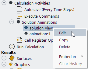
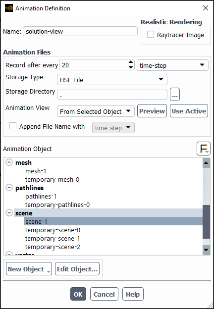
Set how frequently you want the parent dashboard window updated in the Record After Every field.
Update the Storage Type to one of the available image types available in the drop-down list, if you plan to playback the animation or save it once the calculation is complete.
Confirm the remaining settings match your expectations (including the Animation View) and click when you are done.
Important: Only the object included in the solution-view animation definition is updated at a specified interval while Fluent is calculating. Objects in other windows (for example a mesh plot) embedded on the solution view window are not updated as the solution progresses.
Proceed with the remainder of the solution setup. Once the computation is complete, the animation can then be saved in standard video formats, as described in Saving an Animation Sequence.
The following limitations exist for embedded windows:
Save embedded layout in case file option in Preferences:
This option works best (that is, your layout and the parent and child windows will be the same) when you manually create your embedded window dashboard, as described in Manually Embedding Windows. To see the dashboard in a new session, ensure the baselines/parent window is displayed before beginning the calculation.
The layout may not be preserved if you change the layout of the Fluent UI elements (such as collapsing the Outline View or Task Page or by one of the options made available via the Arrange the workspace drop-down list (
 ).
).(Fluent in Workbench) To preserve the Solution View layout, you must select the Use settings changes for current and future calculations. option in the Settings have changed! dialog box that appears when you close your Fluent session.
Context menu options are limited in the embedded windows to the most relevant options. You can swap an embedded window with the primary window (either by double-clicking the embedded window or using the context menu) to access the full context menu options.
Embed in > context menu options (accessed by right-clicking an object in the Outline View tree) are grayed-out when this object is already included in a saved embedded window layout from a previous session.
When saving pictures by using the Save Picture dialog box:
Ensure that the parent window is in focus (and not an embedded window) if you want the entire embedded window dashboard captured.
The border and the window titles of embedded windows will not be included in the saved images.
You can only save 2D images of the embedded window dashboard (that is, JPEG, PPM, TIFF, PNG).
The layout of the embedded window may not remain exactly the same when you swap it with the parent window (by double-clicking or using the context menu) and then swap back.
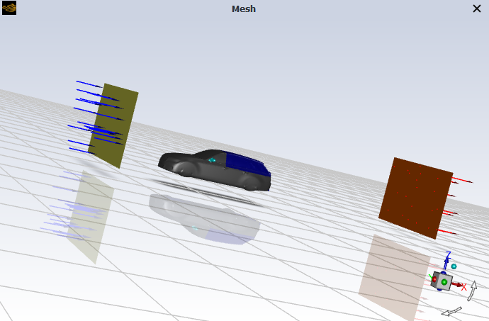
Normally, you can see only one picture at a time in the graphics window, unless you are Displaying a Scene. Sometimes, however, you may want to create an "exploded" view, where results translated or rotated out for the physical domain for enhanced display (see Figure 40.59: Exploded Scene Display of Temperature and Velocity). You can do this by turning on the Overlays option (and clicking ) and using the transform operation in the Scene Description Dialog Box.
![]() View → Graphics
→ Compose...
View → Graphics
→ Compose...
Once overlaying is enabled, subsequent graphics that you generate will be displayed on top of the existing display in the active graphics window. To generate a plot without overlays, you must turn off the Overlays option in the Scene Description Dialog Box (and remember to click ).
When you are overlaying multiple graphics, the captions and color scale that will appear in the latest display are those that correspond to the most recently drawn graphic.
Note that when overlaying is enabled, it will apply to all graphics windows, including those that are not yet open. Turning overlays on and off does so for all graphics windows, not just for the active window. That is, if you enable overlays, open a new graphics window (as described in Managing Multiple Graphics Windows), and then generate two or more graphics in that window, they will be overlaid.
During your Ansys Fluent session, you can open up to 50 graphics windows at one time and they may
be viewed within the application window or in separate windows (sub-window view).
Ansys Fluent can separately open up to an additional 50 windows, referred to as
'Reserved', which contain displays that are generated while the solver is running.
These reserved windows include residuals (Printing and Plotting Residuals), report plots (Report Files and Report Plots), and animation
definitions (Creating an Animation Definition). Reserved windows
are indicated by a grayed-out Fluent icon (![]() ) and they do not offer any context menu options. User-specified
windows are indicated by a Fluent icon (
) and they do not offer any context menu options. User-specified
windows are indicated by a Fluent icon (![]() ) and they provide additional context menu options via
right-click (see examples in Graphics Windows).
) and they provide additional context menu options via
right-click (see examples in Graphics Windows).
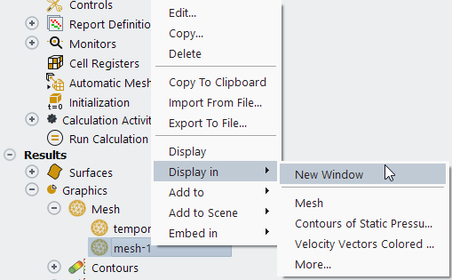
You can open new graphics windows by right-clicking the top of the graphics window tab (or the top of the window if you are in sub-window view) and select New Window. Alternatively, you can display boundaries and graphics objects in a new window by right-clicking them in the Outline View tree and clicking Display in → New Window (as shown in Figure 40.60: Outline View 'Display in' Example. Refer to The Outline View for additional information on the context menu options.
If there are a lot of graphics windows open or if you want to be certain that you are selecting the intended window, you can select the More... context menu option (Display in → More...), which opens the Select Window dialog box (Figure 40.61: The Select Window Dialog Box).
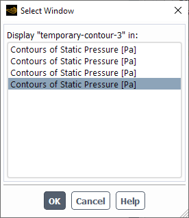
As soon as you select a window from the list, that window is made active. Clicking displays the selected object in the specified graphics window.
When you are viewing graphics windows in sub-window view (rather than tabbed) or if you are using the embedded windows feature (Embedded Graphics Window Dashboards), you may want to synchronize the views so that manipulations performed in one window, such as zooming or panning, are also performed in the other open windows. Refer to Synchronizing Window Views for additional information.
When you have more than one graphics window open, you must identify the active window so that Ansys Fluent will know which one to draw the plot in. Identify the active window by clicking any mouse button in the desired window. This window will remain active until you set a new active window.
You can synchronize two or more open graphics windows so that their views are linked and graphical manipulations (such as panning or zooming) performed in one window are done in the other synchronized windows simultaneously.
There are two ways that you can start and stop the synchronization process:
Click the Synchronize Views toolbar button (
 ). This synchronizes the views of all open graphics
windows to the current view of the active graphics window.
). This synchronizes the views of all open graphics
windows to the current view of the active graphics window.Right-click in the graphics window with the view that you want other graphics windows to match and select either Synchronize > Start or Synchronize > Synchronize all windows from the context menu.
You can then synchronize other graphics windows to the first window by right-clicking in the window and selecting Synchronize > Add this window (assuming you did not select the Synchronize all windows option).
You can disable window synchronization either by clicking the unsynchronize
button in the toolbar (![]() ), which stops the process for all windows, or by
right-clicking the graphics window and selecting Synchronize > Remove
this window, which only removes the selected window from the
synchronization process.
), which stops the process for all windows, or by
right-clicking the graphics window and selecting Synchronize > Remove
this window, which only removes the selected window from the
synchronization process.
Enabled by default when the mesh is displayed, boundary markers allow you to quickly see the flow direction for inlets and outlets in the graphics window. Boundary markers are 2D arrows that point into the model for inlets and out of the model for outlets, as shown in Figure 40.62: Boundary Markers on an Inlet and Outlet.
The boundary markers button in the graphics window toolbar (![]() ) allows you to turn the boundary markers on and off.
) allows you to turn the boundary markers on and off.
You can have greater control over the appearance of the boundary markers in Preferences (accessed by selecting Preferences... from the File ribbon tab).
In Preferences, you can:
Toggle whether boundary markers are enabled for inlets and outlets separately.
Control the relative size of the boundary markers.
Choose the color of the boundary markers.
Specify the maximum number of boundary markers that can be displayed on a surface. (The actual number displayed will be based on this limit and the specified density.)
Control the density of boundary markers on a surface (with values of 0.1 to 1). The larger the value for density, more tightly the arrows can be packed on the surface. A value of 1 means that one boundary marker would be shown per surface facet (assuming the Limit is higher than the number of facets).
Limitations
Boundary markers only work on the mesh display if Outline is selected under Edge Type in the Mesh Display dialog box.
Boundary Markers are not shown for the Pressure Far-Field inlet type.
For 2D cases, boundary markers may be unreliable and could show incorrect directions due to issues with how settings are stored and managed in global and saved graphics objects.
Ansys Fluent graphics include, by default, a caption or legend block that consists of fields of text describing the contents of the graphic, the Ansys Fluent product identification, an axis triad indicating the orientation of the displayed object, a color key defining the correspondence between each color and the magnitude of the plotted variable, and the ANSYS logo. You can turn off the display of the legend and color scale, and/or the axis triad. You can also hide the ANSYS logo. You can also display the colormap on any side of the display window as per convenience. In addition you can also edit the captions directly in the graphics window.
You can enable/disable the display of the Titles, Axes, and Ruler directly in the graphics window by toggling the appropriate icon (refer to Additional Display Options for more information). The Logo and the Colormap are controlled under Layout in the Display Options Dialog Box (Display Options Dialog Box).
![]() Results →
Graphics
Results →
Graphics
![]() Options...
Options...
Use the text interface to enable/disable the captions and color scale individually, and to change the size and position of the captions and color scale.
display →
set → windows
→ text →
display →
set → windows
→ scale →
See the separate Text Command List for details.
Controlling Titles
You can add text, such as your company name, to the title box in multiple
locations using the display/set/titles/ text command
locations. Once you have provided text for one of these locations, you must
ensure that display/set/windows/text/company? is set to
yes, then re-render the display by displaying a graphics object (for example,
mesh, contour, vector, and so on) or by entering
display/re-render in the console.
Alternatively, if you always want your company name or other text displayed in
the title box, you can set the FLUENT_COMPANY
environment variable in the Fluent Launcher equal to your company name or the
desired text, for example, FLUENT_COMPANY=My Example Company
Name. Note that Titles is
disabled by default when you launch Fluent, so you will have to enable
Titles before it will be displayed in the graphics
window.
When captions are displayed in the graphics window, you may choose to modify, delete, or add to the text that appears in the caption box. To do so, click the left mouse button in the desired location. A cursor will appear, and you can then type new text or delete the text that was originally there (using the backspace or delete key). Note that changes to existing text in the caption block will be removed when you draw new graphics in the window (unless you are overlaying multiple graphics in the same window), but text that you add on a previously empty line in the caption block will not be removed until the default caption text makes use of that line.
You can define a title for your problem using the title text command:
display → set → title
The title you define will appear on the top line of the caption, at the far left, in all subsequent plots. It will also be saved in the case file.
Important: You will need to enclose your title in quotation marks (for
example, "
my title
").
You can disable the display of the axis triad by turning off the Axes
Visibility button (![]() ) in the graphics window.
) in the graphics window.
You can disable the display of the ruler by turning off the Ruler
Visibility button (![]() ) in the graphics window.
) in the graphics window.
Note that if your project is 3D, then enabling the ruler automatically changes the view to orthographic so that the ruler markings are relevant for the model.
The graphics window displays a white ANSYS logo in the upper right corner. You may choose between a white (default) or black logo by selecting White or Black from the Color drop-down list under Layout in the Display Options Dialog Box (Display Options Dialog Box).
You can prevent the ANSYS logo from being displayed in the graphics window by disabling the Logo option under Layout.
You can use the Annotate Dialog Box to add text to the graphics window with optional attachment lines. Figure 40.63: Graphics Window with Text Annotation shows an example of a graphics display with annotated text in it.
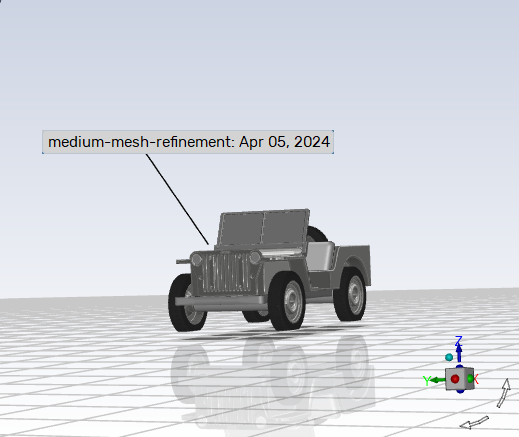
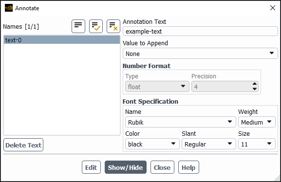
Adding text to the graphics window using the Annotate Dialog Box (Figure 40.64: The Annotate Dialog Box) allows you to control the font and color of the text.
![]() Results → Graphics
Results → Graphics ![]() Annotate...
Annotate...
The steps for adding text are as follows:
Enter the text that you want to add in the Annotation Text field.
(Optional) Select a Value to Append from the drop-down list.
(Flow-time and expressions only) Specify the desired formatting of the flow-time output. You can control the Type and Precision in the Number Format group box.
Under Font Specification, select the font type in the Name drop-down list, the font weight (Medium or Bold) in the Weight drop-down list, the size (in points) in the Size drop-down list, the color in the Color drop-down list, and the slant (Regular or Italic) in the Slant drop-down list.
Click . You will be asked to pick the location in the graphics window where you want to place the text, using the left mouse button.
If you click the mouse button once in the desired location, the text will be placed at that point. Dragging the mouse with the left-mouse-button depressed will draw an attachment line from the point where the mouse was first clicked to the point where it was released. The annotation text will be placed at the point where the mouse button was released.
Important: Annotations are added to a specific graphics window and they are not persisted with the displayed object. If you open a new graphics window, you will not see any annotations listed in the Annotate dialog box.
For animations where you want an annotation to update, you must first Preview the animation object, then add the annotation. When playing back the animation, first close the original graphics window where the animation definition was previewed, since the annotation will still be there and it may give the impression that the annotation is not updating as the animation plays.
Once you have added text to the graphics display, you may change the font characteristics of one or more text items, or delete individual text items.
To modify or delete existing text, follow these steps:
Select the appropriate item in the Names list in the Annotate Dialog Box (Figure 40.64: The Annotate Dialog Box). When you select a name, the associated text will be displayed in the Annotation Text field, and the button becomes the button.
Modify the Font Specification entries as desired, and click to modify the text, or simply click below the Names list to delete the selected text.
Note that if you want to make changes to all current annotation text, you can select all of the Names instead of just one in step 1.
You can move the text by clicking (left mouse button) and dragging the annotation text in the graphics window. If a line is attached, it will move as needed to continue pointing at the original location and text.
Annotation text is associated with the active graphics window and is removed only when the annotations are explicitly cleared. To remove the annotations from the graphics window, you must click in the Annotate Dialog Box. If you draw new graphics in the window without clearing the annotations, they will remain visible in the new display.
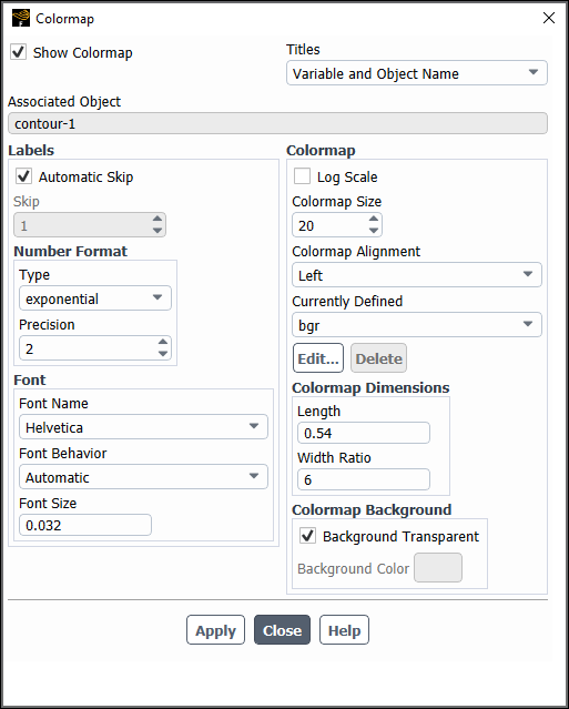
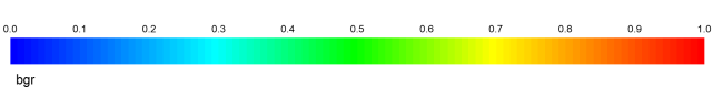
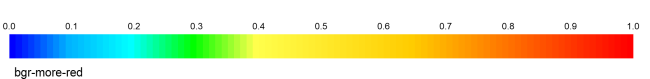
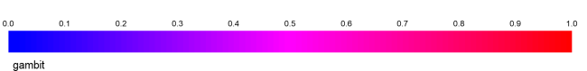
The default colormap used by Ansys Fluent to display graphical data (for example, vectors) ranges from blue (minimum value) to red (maximum value). Additional predefined colormaps are available, and you can also create custom colormaps. To make any changes to the colormap, you will use the Colormap Dialog Box (Figure 40.66: The Colormap Dialog Box).
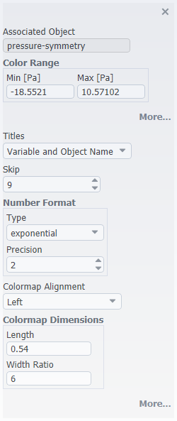
If you have already displayed a graphics object, such as a contour or vector plot, you can double-click the colormap in the graphics window to open Figure 40.67: The Colormap Quick-Edit Panel. This panel lets you quickly change colormap properties directly in the graphics window and the changes are saved as soon as you leave the field you are editing. These properties include the range of values the colormap is covering.
If you want to temporarily hide a colormap from the graphics window, for example, when capturing a picture (Saving Picture Files), you can click the 'X' that appears when hovering over the upper-right corner of the colormap (as shown in Figure 40.65: Temporarily Hiding the Colormap). There is a Show Colormap context menu option (accessed by right-clicking in the graphics window) allowing you to bring back any hidden colormaps.
Note:
You can control many colormap default settings using preferences, including the colormap font, font size, colormap size, location, physical size in the graphics window, number format type and precision, and more. All of the available settings are listed under Colormap Settings in the Graphics branch of Preferences (accessed via File → Preferences...).
Opening the Colormap dialog box from within a graphics object (such as the Contours or Vectors dialog box) provides more options than opening it from the Views ribbon tab or a right-click of the Graphics branch in the Outline View tree).
![]() Results → Graphics
Results → Graphics ![]() Colormap...
Colormap...
When you plot contours, you can temporarily modify the number of colors in the colormap by changing the number of contour levels in the Contours Dialog Box; you will only need to use the Colormap Dialog Box if you want to change other characteristics of the colormap.
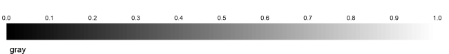
Important: Note that if you are using a gray-scale colormap and you want to save a gray-scale picture, you should save a color picture. When you save a gray-scale picture, Ansys Fluent uses an internal gray scale, not the gray scale specified by the colormap. If you save a color picture, the colormap you selected (that is, your gray scale) will be used.
The following are a list of common terms and definitions used in colormap labels:
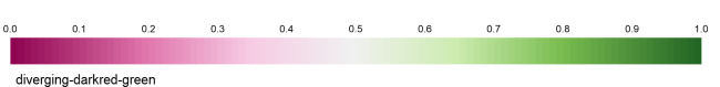
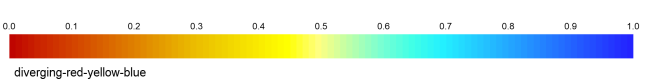
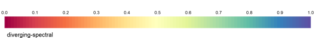
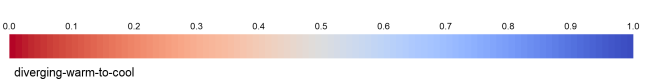
Diverging—when converted to greyscale (for example, when printing) these are bright in the center and darker at the ends.
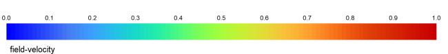
Field—using scenes (Generating a Scene) you can visualize multiple fields within a single plot, such as pressure and temperature. To clearly differentiate the field variables, it is recommended that you use different colormaps for each variable. The field names included in the name of a predefined colormap are meant to indicate the recommended colormap for visualizing a particular variable.
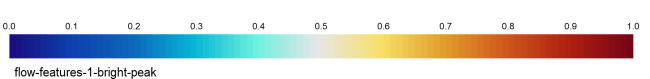
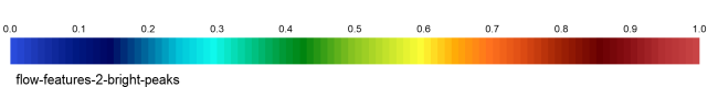
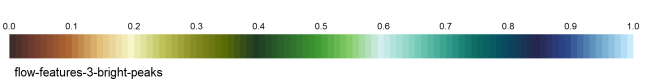
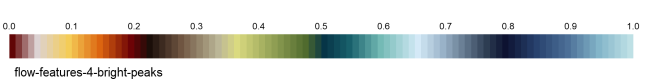
Flow-feature-N-bright-peaks—these are intended to help you identify relevant flow features. N indicates the number of bright peaks in the colormap.
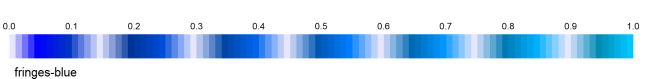
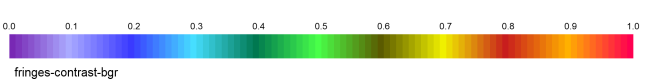
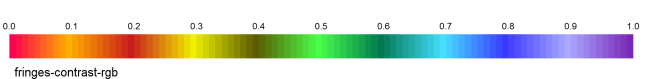
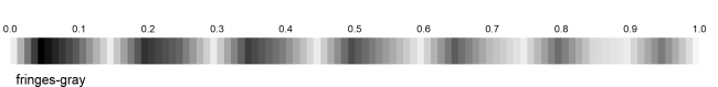
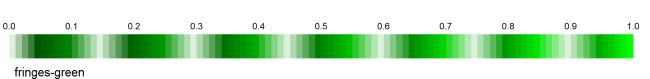
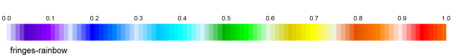
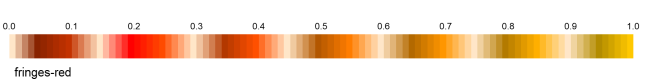
Fringes—brightness alternates multiple times.
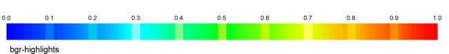
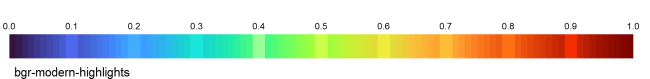
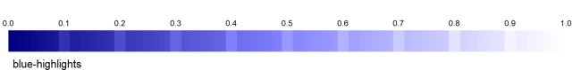
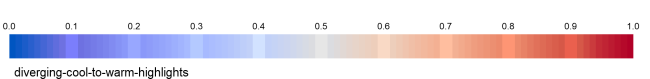
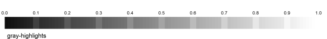
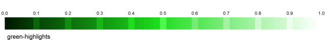
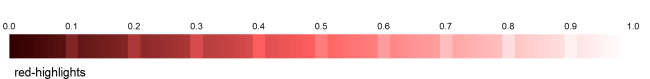
Highlights—used as a suffix. The colormap has 9 highlights, dividing it into 10 levels.
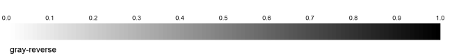
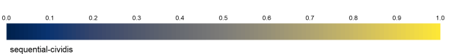
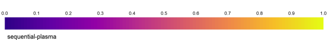
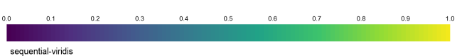
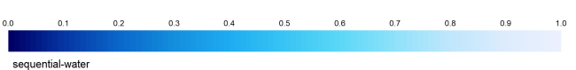
Sequential—when converted to greyscale, these colormaps are dark at the bottom and bright at the top.
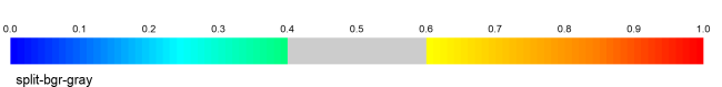
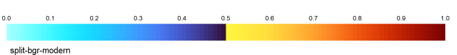
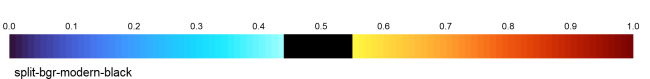
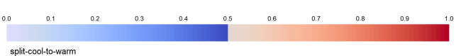
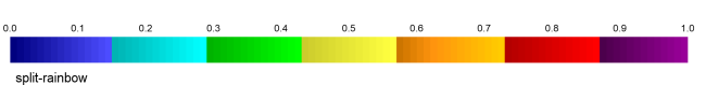
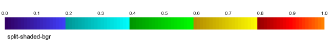
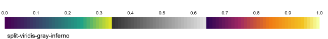
Split—two or more different colormaps in one. When there are two, on eis above the midpoint and one below.
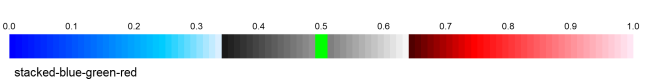
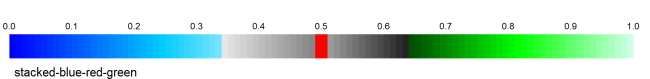
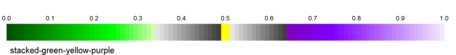
Stacked—three different colormaps stacked. The center one is greyscale. There is a line in a contrasting color at the midpoint.
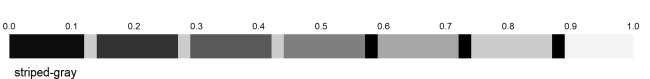
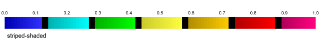
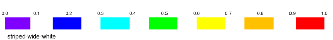
Striped—multiple contrasting stripes to better indicate quantitative values.
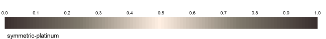
Symmetric—symmetric around the midpoint.
Value—colorful for the indicated value ranges, monochromatic outside the ranges.
The following colormaps are automatically available in Ansys Fluent:
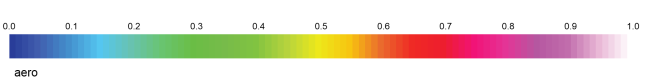
- aero:
- bgr:
- bgr-highlights:
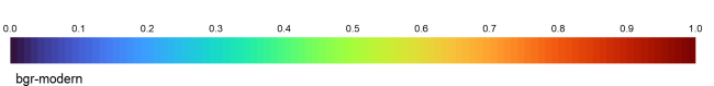
- bgr-modern:
- bgr-modern-highlights:
- bgr-more-red:
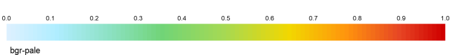
- bgr-pale:
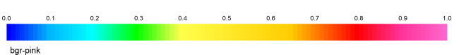
- bgr-pink:
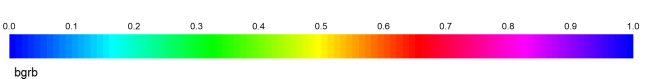
- bgrb:
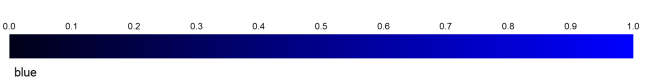
- blue:
- blue-highlights:
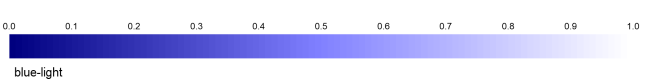
- blue-light:
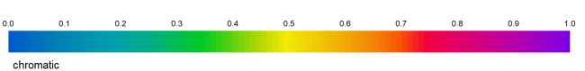
- chromatic:
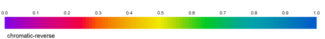
- chromatic-reverse:
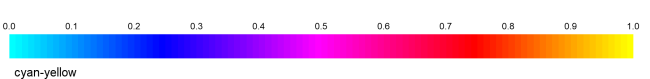
- cyan-yellow:
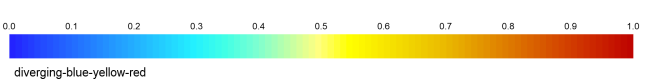
- diverging-blue-yellow-red:
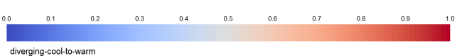
- diverging-cool-to-warm:
- diverging-cool-to-warm-highlights:
- diverging-darkred-green:
- diverging-red-yellow-blue:
- diverging-spectral:
- diverging-warm-to-cool:
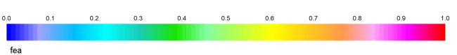
- fea:
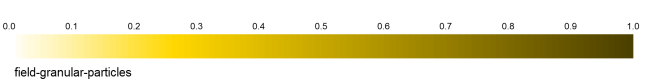
- field-granular-particles:
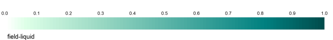
- field-liquid:
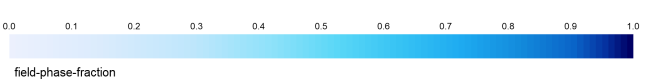
- field-phase-fraction:
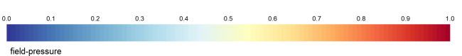
- field-pressure:
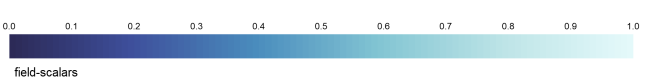
- field-scalars:
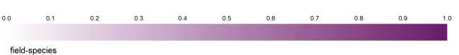
- field-species:
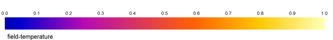
- field-temperature:
- field-velocity:
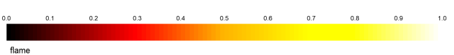
- flame:
- flow-features-1-bright-peak:
- flow-features-2-bright-peaks:
- flow-features-3-bright-peaks:
- flow-features-4-bright-peaks:
- fringes-blue:
- fringes-contrast-bgr:
- fringes-contrast-rgb:
- fringes-gray:
- fringes-green:
- fringes-rainbow:
- fringes-red:
- gambit:
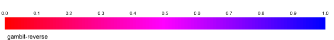
- gambit-reverse:
- gray:
- gray-highlights:
- gray-reverse:
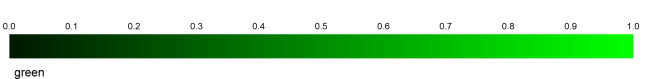
- green:
- green-highlights:
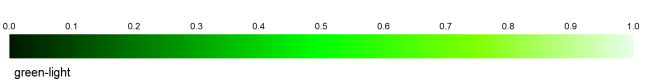
- green-light:
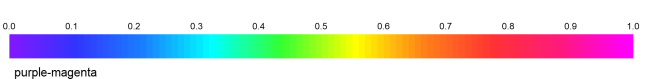
- purple-magenta:
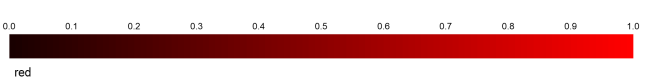
- red:
- red-highlights:
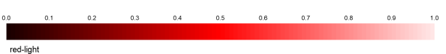
- red-light:
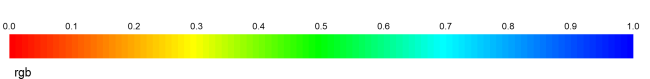
- rgb:
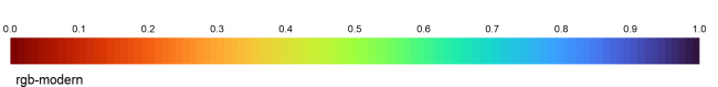
- rgb-modern:
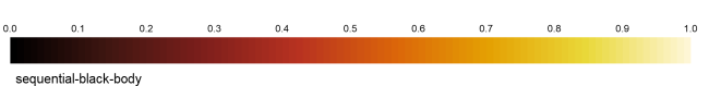
- sequential-black-body:
- sequential-cividis:
- sequential-inferno:
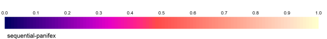
- sequential-panifex:
- sequential-plasma:
- sequential-viridis:
- sequential-water:
- split-bgr-gray:
- split-bgr-modern:
- split-bgr-modern-black:
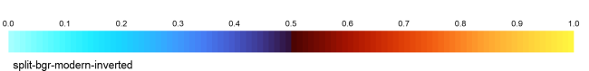
- split-bgr-modern-inverted:
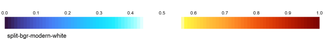
- split-bgr-modern-white:
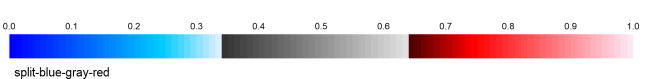
- split-blue-gray-red:
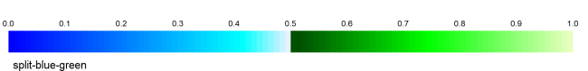
- split-blue-green:
- split-cool-to-warm:
- split-rainbow:
- split-shaded-bgr:
- split-viridis-gray-inferno:
- stacked-blue-green-red:
- stacked-blue-red-green:
- stacked-green-yellow-purple:
- striped-cartoon:

- striped-gray:
- striped-shaded:
- striped-wide-white:
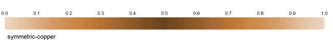
- symmetric-copper:
- symmetric-platinum:
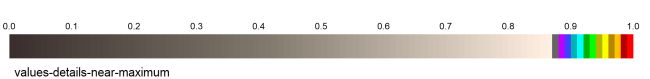
- values-details-near-maximum:
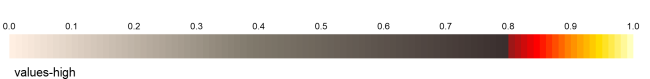
- values-high:
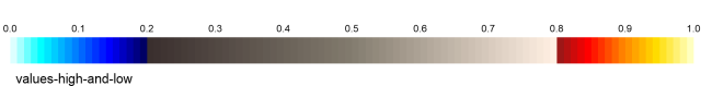
- values-high-and-low:
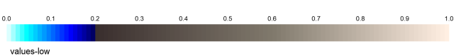
- values-low:
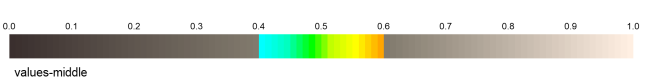
- values-middle:
The number of colors interpolated between the colors in the scale name (for example, between purple and magenta) will depend on the size of the colormap.
The procedure for selecting a new colormap to be used in graphics displays is as follows:
In the Colormap Dialog Box (Figure 40.66: The Colormap Dialog Box), select the desired colormap in the Currently Defined drop-down list. This list will contain all of the colormaps predefined by Ansys Fluent as well as any custom colormaps that you have created as described in Creating a Customized Colormap.
Set the colormap size and scale as described in Specifying the Colormap Size and Scale.
Click to update the current graphics display with the new colormap. All future displays will use the newly selected colormap and options.
Once you have selected the desired colormap from the Currently Defined list, you may modify the Colormap Size (recommended that you use multiples of 10). This value is the number of distinct colors in the color scale.
You can choose to use a logarithmic scale instead of a decimal scale by turning on the Log Scale option. With a log scale, the color used in the graphics display will represent the log of the value at that location in the domain. The values represented by the colors will, therefore, increase exponentially.
You can control the appearance of the colormap in the graphics window by modifying the Length and Width Ratio fields under Colormap Dimensions in the Colormap Dialog Box.
Note: If you are looking to control the "physical" size of the colormap, that is, where and how large it appears in the graphics window, then you can use the Alignment, Length and Width Ratio controls (as well as others) under Colormap Settings the Appearance branch of Preferences (File>Preferences...).
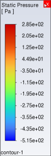
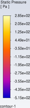
You can change the format of the labels that define the color divisions at the left of the graphics window using the controls under the Number Format heading in the Colormap Dialog Box.
To display the real value with an integral and fractional part (for example, 1.0000), select float in the Type drop-down list. You can set the number of digits in the fractional part by changing the value of Precision.
To display the real value with a mantissa and exponent (for example, 1.0e-02), select exponential in the Type drop-down list. You can define the number of digits in the fractional part of the mantissa in the Precision field.
To display the real value with either float or exponential form, depending on the size of the number and the defined Precision, choose general in the Type drop-down list.
You can control which titles are included with the colormap as well as customize the number of values displayed on the colormap. The default titles include the variable name, units, and the name of the associated graphics object. The default number of labels that appear alongside the colormap is determined automatically based on the screen resolution.
Titles are controlled via the Titles drop-down list, which contains the following options:
Variable and Object Name—both the variable name and the associated graphics object are listed with the colormap, along with the units.
Variable Only—only the variable name and the units are listed with the colormap.
None—only the units are listed with the colormap.
Controlling the number of lables:
To change the number of labels that appear alongside the colormap, disable Automatic Skip in the Colormap Dialog Box and specify the Skip. The total number of labels displayed will then be determined by the Skip and Colormap Size fields.
To demonstrate what effect this command has on the display, enter a value of
10for Skip (note that the value entered must be an integer). This will result in 9 intermediate labels being skipped (assuming you maintain the default colormap size) with the first and the last colormap values always being displayed (Figure 40.68: The Colormap with All Titles and Skipped Labels).To reset the original colormap display, simply select Automatic Skip.
You can create your own colormap by manipulating the existing “color stops” and by adding more of them. A color scale is created by linear interpolation between the color stops. The color, number, and position of the anchor colors will therefore control the description of the colormap. By increasing the number of color stops, you can increase the total number of colors and obtain a color scale that changes more gradually. The procedure is as follows:
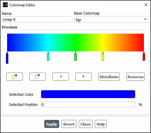
Click in the Colormap Dialog Box to open the Colormap Editor Dialog Box (Figure 40.69: The Colormap Editor Dialog Box).
Provide a name for the custom colormap you are creating.
Select the colormap you want to use as a starting point for your custom colormap from the Base Colormap drop-down list.
Drag the colormap stops to customize the color distribution of the colormap.
Click "insert stop" (
 ) to add a new stop next to the selected
stop.
) to add a new stop next to the selected
stop.Alternatively, you can click in the colormap to add new stops; the color of the new stop will be the same as the location you click.
Click "remove stop" (
 ) to remove the selected color stop.
You can either select color stops directly or you can switch which one is selected using the left and right arrows (
 and
and  ).
).You can change the color of the selected stop by clicking in the Selected Color field and choosing an alternate color from the Select Color dialog box.
Alternatively, you can double-click a color stop to open the Select Color dialog box to change the color for that color stop.
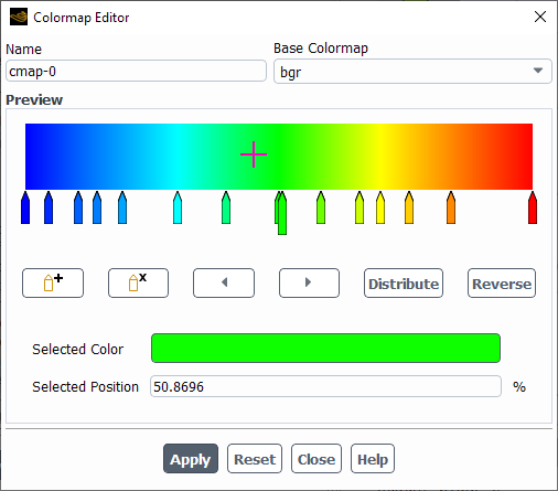
Instead of dragging the color stops, you can enter the location of the stop on the colormap in the Selected Position field.
(Optional) Click to evenly distribute the color stops on the colormap.
Important: The total number of colors must not be less than the number of anchor points.
(Optional) Click to reverse the order of the colors in the colormap.
Click to save the custom colormap.
(Optional) Click to reset the current display to the Base Colormap.
Custom colormap definitions will be saved in the case file.
The following are a list of resources used in the implementation of colormaps in Ansys Fluent.
[1] "Color Map Advice for Scientific Visualization". Kenneth Moreland. 2015,. https://www.kennethmoreland.com/color-advice/.
[2] "Wavelets and Turbulence". http://wavelets.ens.fr/.
[3] "Choice of Representation Modes and Color Scales for Visualization in CFD". Science and Art Symposium 2000. Kluwer. 91–100. 2000.
[4] "Visualizing Science: How Color Determines What We See". Eos, Science News by AGU. May 21, 2020.
[5] "CFD Post Processing". Google AI Blog. August 20, 2019. https://ai.googleblog.com/2019/08/turbo-improved-rainbow-colormap-for.html.
[6] "Turbo, An Improved Rainbow Colormap for Visualization". Race Tech Magazine. February 5, 2019. https://www.racetechmag.com/2019/02/willem-toet-explains-cfd-post-processing/.
In Ansys Fluent you can add lights with a specified color and direction to your display. These lights can enhance the appearance of the display when it contains 3D geometries. By default one light is defined. You can enable the effect of the existing light(s) using the Display Options Dialog Box or the Lights Dialog Box, and you can add new lights using the Lights Dialog Box.
You can control default lighting behavior using the settings listed under Lighting in the Graphics branch of Preferences (Setting User Preferences/Options). Controls are available for:
Lighting method
Headlight behavior and intensity
Ambient light intensity
Important: While the best lighting method for most situations is handled automatically, if you are displaying mesh faces only, edges may appear rounded due to a third-party issue. To resolve this issue, you can either enable Edges in the Mesh Display Dialog Box, or you can select the Flat lighting method, either from the drop-down list in the View ribbon tab or in the Lighting Method drop-down list under Lighting in the Graphics branch of Preferences.
Lighting is handled automatically by default, however you can turn the lights off and control the lighting method manually if desired using the Display Options Dialog Box.
![]() Results → Graphics
Results → Graphics ![]() Options...
Options...
The Lights On option is enabled with the method set to Automatic by default, but you can disable Lights On and change the method from the Lighting drop-down. Once you have changed the method you must click for the change to take effect.
The lighting interpolation methods include: Flat, Gouraud and Phong. Flat is the most basic method: there is no interpolation within the individual polygonal facets. Gouraud and Phong have smoother gradations of color because they interpolate on each facet.
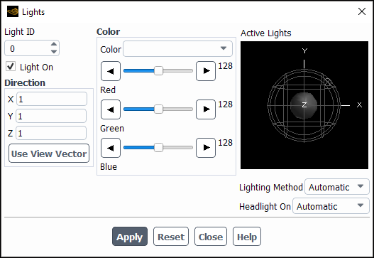
You can also control lighting effects using the Lights Dialog Box (Figure 40.71: The Lights Dialog Box).
![]() Results → Graphics
Results → Graphics ![]() Lights...
Lights...
The headlight provides constant lighting effects in the direction of view and it is controlled automatically by default to optimize the appearance for the type of graphics object being displayed. This option has the effect of a light source directly in front of the model, no matter what orientation the model is viewed in. You can control the headlight manually be setting Headlight On to On or Off using the drop-down in the Lights Dialog Box.
Fluent controls the lighting method automatically by default, optimizing the appearance of the graphics for the object being displayed. You have the option to control the method manually by selecting Flat, Gouraud, or Phong from the Lighting Method drop-down list. These methods are described in the previous section. Click to see any changes made to the lighting effects in the active graphics window.
You can control individual lights in the Lights Dialog Box (Figure 40.71: The Lights Dialog Box). The Lights Dialog Box enables you to create a light and then turn it off without deleting it. In this way, you can retain lights that you have defined previously but do not want to use at present.
![]() Results → Graphics
Results → Graphics ![]() Lights...
Lights...
(You can also open the Lights Dialog Box by clicking in the Display Options Dialog Box.)
By default, light 0 is defined to be dark gray with a direction of (1,1,1). A light source is a distant light, similar to the sun. The direction (1,1,1) means that the rays from the light will be parallel to the vector from (1,1,1) to the origin. To create an additional light (for example, light 1), follow the steps listed below.
Increase Light ID to a new value (for example,
1).Enable the Light On check box.
Define the light color by entering a descriptive string (for example,
lavender) in the Color field, or by moving the Red, Green, and Blue sliders to obtain the desired color. The default color for all lights is dark gray.Specify the light direction by doing one of the following:
Enter the (X, Y, Z) Cartesian components under Direction.
Click the middle mouse button in the desired location on the sphere under Active Lights. (You can also move the light along the circles on the surface of the sphere by dragging the mouse while holding down the middle button.) You can rotate the sphere by pressing the left mouse button and moving the mouse (like a trackball).
Use your mouse to change the view in the graphics window so that your position in reference to the geometry is the position from which you would like a light to shine. Then click to update the X,Y,Z fields with the appropriate values for your current position and update the graphics display with the new light direction. This method is convenient if you know where you want a light to be, but you are not sure of the exact direction vector.
Repeat steps 1–4 to add more lights.
When you have defined all the lights you want, click to save their definitions.
To remove a light, enter the ID number of the light to be removed in the Light ID field and then clear the Light On check box. When a light is turned off, its definition is retained, so you can easily add it to the display again at a later time by selecting the Light On check box. For example, you may want to define three different lights to be used in different scenes. You can define each of them, and then enable only one or two at a time, using the Light ID field and the Light On check box. Once you have made all the desired modifications to the lights, remember to click to save the changes.
If you have made changes to the light definitions, but you have not yet clicked , you can reset the lights by clicking . All lighting characteristics will revert to the last saved state (that is, the lighting that was in effect the last time you opened the dialog box or clicked on ).
Depending on the objects in your display window and what kind of graphics hardware and software you are using, you may want to modify some of the rendering parameters listed below. All are listed under the Rendering heading in the Display Options Dialog Box (Display Options Dialog Box).
![]() Results → Graphics
Results → Graphics
![]() Options...
Options...
After making a change to any of these rendering parameters, click to update how new graphics objects will appear. Note that some changes, such as those to line width and the logo are updated in all applicable graphics windows once you click .
- Line Width:
By default, all lines drawn in the display have a thickness of 1 pixel. If you want to increase the thickness of the lines, increase the value of Line Width.
- Point Symbol:
By default, nodes displayed on surfaces and data points on line or rake surfaces are represented in the display by a
+sign inside a circle. If you want to modify this representation (for example, to make the nodes easier to see), you can select a different symbol in the Point Symbol drop-down list.- Animation Options:
There are two animation options that you can choose from. They are as follows:
- All
uses a solid-tone shading representation of all geometry during mouse manipulation.
- Wireframe
uses a wireframe representation of all geometry during mouse manipulation. If your computer has a graphics accelerator, you may not want to use this option; otherwise, the mouse manipulation may be very slow.
- Double Buffering:
Enabling the Double Buffering option can dramatically reduce screen flicker during graphics updates. Note, however, that if your display hardware does not support double buffering and you turn this option on, double buffering will be done in software. Software double buffering uses extra memory.
- Front Faces Transparent:
This option enables you to turn off the display of outward pointing faces of shells or meshes. This is sometimes useful for displaying both sides of a slit wall. By default, when you display a slit wall, one side will “bleed” through to the other. When you enable the Front Faces Transparent option, the display of a slit wall will show each side distinctly as you rotate the display. This option can also be useful for displaying two-sided walls (that is, walls with fluid or solid cells on both sides). Please note, however, that enabling it can also hides some unintended surfaces on certain viewing angles, e.g. while displaying Contours, it might be visible only from one side of the surface and not from the other
- Hidden Surface Removal:
If you do not use hidden surface removal, Ansys Fluent will not try to determine which surfaces in the display are behind others; it will display all of them, and a cluttered display will result for most 3D mesh displays. For most 3D problems, therefore, you should enable the Hidden Surface Removal option. You should turn this option off (for optimal performance) if you are working with a 2D problem or with geometries that do not overlap.
You can choose one of the following methods for performing hidden surface removal in the Hidden Surface Method drop-down list. These options vary in speed and quality, depending on the device you are using.
- Hardware Z-buffer
is the fastest method if your hardware supports it. The accuracy and speed of this method is hardware-dependent. Note that if this method is not available on your computer, selecting it will cause the Software Z-buffer method to be used.
- Painters
will show fewer edge-aliasing effects than Hardware-Z-buffer. This method is often used instead of Software-Z-buffer when memory is limited.
- Software Z-buffer
is the fastest of the accurate software methods available (especially for complex scenes), but it is memory-intensive.
- Z-sort only
is a fast software method, but it is not as accurate as Software-Z-buffer.
If you need to know which graphics driver you are using and what graphics hardware it recognizes, you can click in the Display Options Dialog Box. The graphics device information will be printed in the text (console) window.
Important: Ensure your graphics driver is up-to-date to avoid issues with graphics displays (such as the display coming upside-down).