


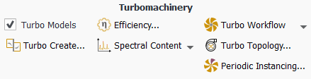
In addition to the many graphics tools already discussed, Ansys Fluent also provides turbomachinery-specific postprocessing features that can be accessed once you have defined the topology of the problem. Information on postprocessing for turbomachinery applications is provided in the following sections:
In order to establish the turbomachinery-specific coordinate system used in subsequent postprocessing functions, Ansys Fluent requires you to define the topology of the flow domain. The procedure for defining the topology is described further in this section, along with details about the boundary types.
The current implementation of the turbomachinery topology definition for postprocessing is no longer limited to one row of blades at a time. If your geometry contains multiple rows of blades, you can define all turbomachinery topologies simultaneously. You can name and/or manage all topologies and perform various turbomachinery postprocessing tasks on a single topology or on all topologies at once.
Important: The turbo coordinates can only be generated properly if the correct rotation axis is specified in the boundary conditions dialog box for the fluid zone (see Specifying the Rotation Axis).
To define the turbomachinery topology in Ansys Fluent, you will use the Turbo Topology Dialog Box (Figure 14.24: The Turbo Topology Dialog Box).
![]() Domain
→ Turbomachinery → Turbo
Topology...
Domain
→ Turbomachinery → Turbo
Topology...
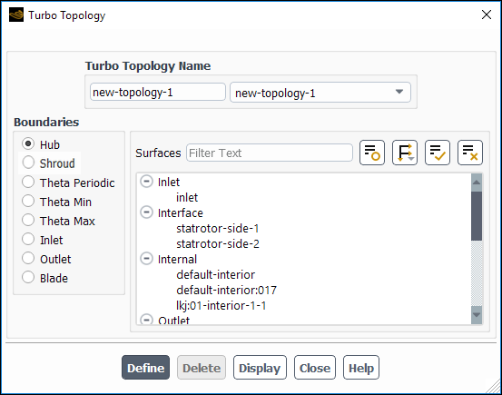
The procedure for defining topology for your turbomachinery application are as follows:
Select a boundary type under Boundaries (for example, Hub in Figure 14.24: The Turbo Topology Dialog Box). The boundary types are described in detail in Boundary Types.
In the Surfaces list, choose the surface(s) that represent the boundary type you selected in step 1.
If you want to select several surfaces of the same type, click
 and select Surface Type under Group
By, which organizes the surfaces in a tree view that is grouped by surface
type.
and select Surface Type under Group
By, which organizes the surfaces in a tree view that is grouped by surface
type.Another shortcut is to use the Filter Text entry box to filter the Surfaces list to show only the surfaces that match the pattern you enter. For additional information on using the Filter Text entry box, see Filter Text Entry Boxes.
Repeat the steps 1 and 2 for all the boundary types that are relevant for your model.
Enter a name in the Turbo Topology Name field or keep the default name.
Click Define to complete the definition of the boundaries.
Ansys Fluent will inform you that the turbomachinery postprocessing functions have been activated.
Specify a position vector that is defined as
 . This position vector should be outside the domain, for example, if
your domain lies in the first and second quadrant, specify negative
. This position vector should be outside the domain, for example, if
your domain lies in the first and second quadrant, specify negative  -axis as the zero
  line. This will ensure that there is no discontinuity in angular
coordinates within the domain. This can be done using the
line. This will ensure that there is no discontinuity in angular
coordinates within the domain. This can be done using the
display/set/zero-angle-dircommand.Default zero
 line is
  -axis. If this axis passes through the domain, you should define the
zero
-axis. If this axis passes through the domain, you should define the
zero  line, so as to satisfy above criteria.
To view a defined topology, select the topology from the Turbo Topology Name drop-down list and click . The defined topology is shown in the active graphics window. This enables you to visually check the boundaries to ensure that you have defined them correctly.
To edit a defined topology, select the topology from the Turbo Topology Name drop-down list, make the appropriate changes and click Modify.
To remove a defined topology, select the topology from the Turbo Topology Name drop-down list and click Delete.
Important: Note that the topology setup that you define will be saved to the case file when you save the current model. Thus, if you read this case back into Ansys Fluent, you do not need to set up the topology again.
However, use of a boundary condition file to set the turbo topology for two similar cases may not work properly. In that case you need to set the turbo topology manually.
Note: From Fluent 2020 R1 onwards, turbo topology TUI access can be
found at define/turbo-model/turbo-topology.
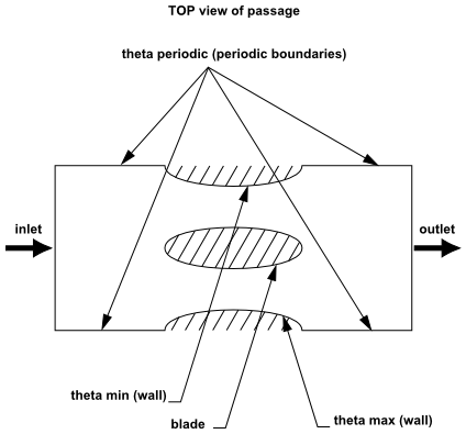
The boundaries for the turbomachinery topology are as follows (see Figure 14.25: Turbomachinery Boundary Types):
- Hub
is the wall zone(s) forming the lower boundary of the flow passage (generally toward the axis of rotation of the machine).
- , Shroud
is the wall zone(s) forming the upper boundary of the flow passage (away from the axis of rotation of the machine).
- Theta Periodic
is the periodic boundary zone(s) on the circumferential boundaries of the flow passage.
- Theta Min
and Theta Max are the wall zones at the minimum and maximum angular (
 ) positions on a circumferential boundary.
- Inlet
is the inlet zone(s) through which the flow enters the passage.
- Outlet
is the outlet zone(s) through which the flow exits the passage.
- Blade
is the wall zone(s) that defines the blade(s) (if any). Note that these zones cannot be attached to the circumferential boundaries. For this situation, use Theta Min and Theta Max to define the blade.
After completing the turbo topology definition detailed in Defining the Turbomachinery Topology, the following turbomachinery-specific variables are available for postprocessing in Ansys Fluent:
These variables are contained in the Mesh... category of the variable selection drop-down list. See Field Function Definitions for their definitions.
Turbomachinery postprocessing commonly requires viewing contour and vector plots on turbo surfaces. As a prerequisite, you must first follow the instructions in Defining the Turbomachinery Topology to enable the Turbomachinery-Specific Variables that are used when creating a turbo surface.
Turbo surfaces are created using the Iso-Surface Dialog Box. The Turbomachinery-Specific Variables are available under the Mesh... category for the Surface of Constant drop-down list. For details on creating iso-surfaces, see Iso-surfaces.
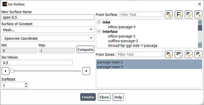
The turbo surfaces will be used to display contours or velocity vectors. It is recommended that you create an iso-surface for each zone separately.
In turbomachinery analysis, it is common that only a portion of the machine is modeled. Therefore, in order to visualize the periodic repeating pattern of a turbomachine, you can use Periodic Instancing to replicate passages around an axis.
Periodic Instancing is accessed from the Turbomachinery ribbon:
![]() Domain
→ Turbomachinery → Periodic
Instancing...
Domain
→ Turbomachinery → Periodic
Instancing...
For more information on Periodic Instancing, see Mirroring and Periodic Repeats and Periodic Instancing Dialog Box.
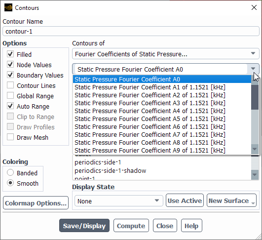
Fluent provides a post-processing Fourier coefficient visualization capability that is
available for all transient cases when Turbo Models is enabled. This
feature supports the accumulation of the following flow variables: static pressure,
temperature, velocity components, turbulent kinetic energy, turbulent dissipation rate
( ), and specific dissipation rate (
 ).
).
The real representation of Fourier coefficients is used and the following
 and
and  are provided in the list of variables available to postprocess. This
representation allows for multiple (M) base frequencies to be captured (
are provided in the list of variables available to postprocess. This
representation allows for multiple (M) base frequencies to be captured ( ), each having its own harmonic content represented by
  . The Fourier coefficient accumulation method used is based on the moving
averages. Its equivalent closed period integration form is given below where the
integration period
. The Fourier coefficient accumulation method used is based on the moving
averages. Its equivalent closed period integration form is given below where the
integration period  must be the common period between all frequencies captured.
Fourier coefficient definitions
 | (14–15) |
The reconstructed signal  can then be written as:
 | (14–16) |
and is provided as a Fourier related variable.
Additional variables available for post-processing are as follows:
 | (14–17) |
 | (14–18) |
where for example  is the time step change in coefficient
  .
.
Utilizing General Fourier Coefficient Postprocessing requires the following pre-requisites.
Turbo Model must be enabled.
 Domain →
Turbomachinery →
Domain →
Turbomachinery →
Turbomachinery Description must be complete. For details, see Turbomachinery Description.
The Run Calculation parameters must be specified using a Fixed time advancement method. It is recommended you use either the Frequency-Based or Period-Based time advancement method and it is required to use a sufficiently small timestep to run the phase-lag method. To accomplish this, you should specify the frequency or period to match the disturbance and then ensure a sufficiently high Time Steps per Period (such as 40). For details, see Configuring Run Calculation Settings.
There are two distinct scenarios for general Fourier coefficient postprocessing:
General cases which include periodic sector or full-wheel simulations for which there are three use-cases: Inlet/outlet disturbance, blade flutter, and transient-rotor-stator
This can be used to help visualize the state of the harmonic content of any transient-periodic turbomachinery simulation.
To make this implementation more general, separate controls are provided to define the spectral description of the postprocessing Fourier coefficients so that you can have different spectral content for each if desired.
Phase-lag single passage cases for which there are two use-cases: Inlet/outlet disturbance and blade flutter
Although these cell-zone-based Fourier coefficients are not strictly the same as those used in the Phase-lag boundary condition, they provide a good approximation of their state if the same spectral content is used as in the Phase-lag boundary. If the Phase-lag boundary was previously defined the first prompt when using the text command asks if the same spectral settings are to be used for the post-processing Fourier coefficients. The manual TUI method of enabling this is given below:
/define/turbo-models/create-graphics-spectral-content
Copy from phase lag spectral description? [yes]
More details on the setup of this option and on the more general user-defined methods of defining graphical spectral content are given below in Creating Graphics Spectral Content.
There are two methods for creating spectral content for Fourier coefficient postprocessing/
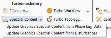
From the Turbomachinery Ribbon
Domain →
Turbomachinery →
There are two entries in the drop down menu as shown in Figure 14.27: Options for Spectral Content in the Turbomachinery Ribbon.
Update Graphics Spectral Content from Phase Lag Data - copies the spectral content from the phase-lag spectral content to the graphics spectral content identically. This will be the most used method to provide the spectral content for the post-processing Fourier coefficients.
Update Graphics Spectral Content from Disturbances - Derive the spectral content from the disturbances that are defined. For inlet/outlet type disturbances, the frequency is derived from the
NumberSectors360parameters provided in any inlet or outlet boundary profile files. For details, see Inlet/Outlet Disturbance Specific Phase-lag Method Workflow. For blade flutter use cases, the frequency associated to the mode-shape that is attached to the fluttering blade is used.
In cases that don't comply with the ribbon option, you have the option to manually create graphics spectral content using the following text command:
/define/turbo-model/create-graphics-spectral-contentThis commands prompts for all the required input to specify the frequencies associated with each disturbance of the simulation in each blade row. If you chose to not use the default number of Fourier harmonics for each fundamental frequency in the specifying spectral options step, you are prompted here to list the desired harmonics for each frequency in the simulation. The frequencies can be specified as disturbances where it will be computed using the input number of sectors in the 360-degree machine and a reference frame. A sample session is shown below:
/define/turbo-model/create-graphics-spectral-content
Add disturbances/frequencies manually? [no] yes
List of all rows: (row-1)
Enter the list of rows to add disturbances/frequencies: (1) [row-1]
Enter the number of disturbances/frequencies for row "row-1": [0] 1
For disturbance/frequency #1:

--> Enter type (1= blade passing disturbance, 2= real frequency in [Hz], 3= blade flutter disturbance): [-1] 1
--> Enter the reference frame associated with this disturbance/frequency Available: ("rotating" "global")

Reference Frame: [] rotating

--> Enter the number of sectors in 360 deg. associated with this disturbance: [0] 19
Calculate modal influence coefficients? [no] no
There are additional settings found under the console command
/define/turbo-model/graphics-extra-settings for changing
defaults associated with spectral content creation of the graphics/post-processing Fourier
coefficients. In most cases, the default values are sufficient and need not be changed. A
sample dialog is shown below.
/define/turbo-model> graphics-extra-settings
Fourier coefficients relaxation [1] 1
Number of initialization cycles [0] 0
Use the default number of Fourier harmonics for each fundamental frequency? [yes] yes
Enter the default number of Fourier harmonics of each fundamental frequency: [10]
The following options are available:
Fourier coefficients relaxationUnder-relaxation constant to be applied to Fourier coefficient accumulation. Current default is 1.0 but a lower value could be used to improve robustness if required.
Number of initialization cyclesNumber of periods to run the simulation using a “periodic like boundary condition” before starting Phase-lag. Permits delaying the onset of Phase-lag to have a better initial guess for the Fourier coefficients which improves robustness at start-up.
Use the default number of Fourier harmonics for each fundamental
                frequency?
By default, uses the default number of harmonics for each fundamental base frequency. Alternatively, you can specify a list of harmonics for each fundamental frequency in the simulation.
Enter the default number of Fourier harmonics of each fundamental
                frequency
A harmonic number to be applied as default to all the base frequencies in the simulation [defaults to 10].
If the case is multi-row, you can specify a frequency selection algorithm option. This provides an easier way to select the fundamental base frequency for each row.
Enter the multi-row frequency selection algorithm option
(1- nearest neighbors, 2- extended neighbors, 3- user-selected)
Nearest neighborsFrequencies related to the component immediately upstream and downstream of the current component.
Extended neighborsAll possible frequency contributions (all rotors see the frequencies from all the stators and vice-versa).
User selectedYou are prompted for the base frequency to include in each blade row.
There are also additional commands to list, append, and delete postprocessing spectral content:
/define/turbo-model/list-graphics-spectral-content
/define/turbo-model/append-graphics-spectral-content
/define/turbo-model/delete-graphics-spectral-content
With Turbo Models enabled, you have the option to write circumferential-averaged profiles. Circumferential-averaged profiles are available for flow variables on various surfaces including inlet, outlet, interfaces, planes, iso-surfaces, and iso-clips. The determination of the profile type (radial or axial) is internally based on the specific type of machine. For more details, see Writing Circumferential-Averaged Profiles.
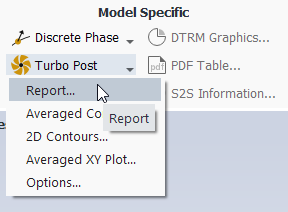
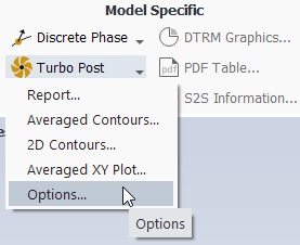
After the turbo topology has been defined, as described in Defining the Turbomachinery Topology, you can access various Turbo Post applications.
![]() Results → Model
Specific → Turbo Post
Results → Model
Specific → Turbo Post
Once you have defined your turbomachinery topologies, as described in Defining the Turbomachinery Topology, you can report a number of turbomachinery quantities, including mass flow, swirl number, torque, and efficiencies.
To report turbomachinery quantities in Ansys Fluent, you will use the Turbo Report Dialog Box (Figure 14.29: The Turbo Report Dialog Box).
![]() Results → Model
Specific → Turbo Post
→ Report...
Results → Model
Specific → Turbo Post
→ Report...
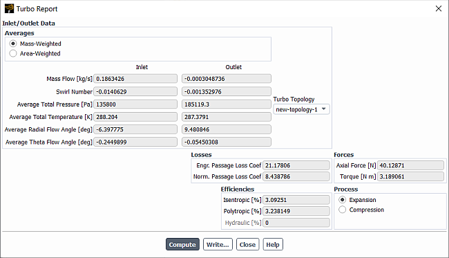
The procedure for using this dialog box is as follows:
Under Averages, specify whether you want to report Mass-Weighted or Area-Weighted averages.
Under Turbo Topology, specify a predefined turbomachinery topology from the drop-down list.
Under Process, specify whether to compute the efficiency for the flow Expansion (for example, in a turbine) or Compression (for example, in a pump or compressor).
Click . Ansys Fluent will compute the turbomachinery quantities as described below, and display their values.
If you want to save the reported values to a file, click Write... and specify a name for the file in The Select File Dialog Box.


The area-averaged total pressure is defined as follows:
 | (14–21) |
where  is the total pressure and
  is the area of the inlet or outlet.
The mass-averaged total pressure is defined as follows:
 | (14–22) |


The area-averaged total temperature is defined as follows:
 | (14–23) |
where  is the total temperature and
  is the area of the inlet or outlet.
The mass-averaged total temperature is defined as follows:
 | (14–24) |


The area-averaged flow angles are defined as follows:
 | (14–25) |
 | (14–26) |
in the tangential direction, where  ,
,  , and
, and  represent the axial, radial, and tangential velocities,
respectively.
represent the axial, radial, and tangential velocities,
respectively.
The mass-averaged flow angles are defined as follows:
 | (14–27) |
 | (14–28) |
The engineering loss coefficient is defined as follows:
 | (14–29) |
| where, | |
 = the mass-averaged total pressure at the inlet = the mass-averaged total pressure at the inlet | |
 = the mass-averaged total pressure at the outlet = the mass-averaged total pressure at the outlet | |
 = the density of the fluid = the density of the fluid | |
 = the mass-averaged velocity magnitude at the inlet = the mass-averaged velocity magnitude at the inlet |
The normalized loss coefficient is defined as follows:
 | (14–30) |


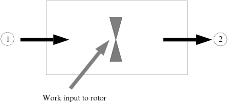
The definitions of the efficiencies for compressible and incompressible flows in pumps and compressors are described in this section. Efficiencies for turbines are described later in this section. Consider a pumping or compression device operating between states 1 and 2 as illustrated in Figure 14.30: Pump or Compressor. Work input to the device is required to achieve a specified compression of the working fluid.
Assuming that the processes are steady state, steady flow, and that the mass flow rates are equal at the inlet and outlet of the device (no film cooling, bleed air removal, and so on), the efficiencies for incompressible and compressible flows are as described in the following subsections.
For devices such as liquid pumps and fans (2D boundaries or 3D cell zones) at low speeds, the working fluid can be treated as incompressible. The efficiency of a pumping process with an incompressible working fluid is defined as the ratio of the head rise achieved by the fluid to the power supplied to the rotor/impeller. This can be expressed as follows:
 | (14–33) |


This definition is sometimes called the “hydraulic efficiency”. Often, other efficiencies are included to account for flow leakage (volumetric efficiency) and mechanical losses along the transmission system between the rotor and the machine providing the power for the rotor/impeller (mechanical efficiency). Incorporating these losses then yields a total efficiency for the system.
For gas compressors that operate at high speeds and high pressure ratios, the compressibility of the working fluid must be taken into account. The efficiency of a compression process with a compressible working fluid is defined as the ratio of the work required for an ideal (reversible) compression process to the actual work input. This assumes the compression process occurs between states 1 and 2 for a given pressure ratio. In most cases, the pressure ratio is the total pressure at state 2 divided by the total pressure at state 1. If the process is also adiabatic, then the ideal state at 2 is the isentropic state.
From the foregoing definition, the efficiency for an adiabatic compression process can be written as
 | (14–34) |


If the specific heat is constant, Equation 14–34 can also be expressed as
 | (14–35) |


 | (14–36) |
where  is the ratio of specific heats specified in the Reference Values Task Page.
The efficiency can be written in the compact form
 | (14–37) |
Note that this definition requires data only for the actual states 1 and 2.
Compressor designers also make use of the polytropic efficiency when comparing one compressor with another. The polytropic efficiency is defined as follows:
 | (14–38) |
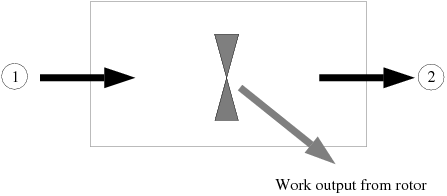
Consider a turbine operating between states 1 and 2 in Figure 14.31: Turbine. Work is extracted from the working fluid as it expands through the turbine. Assuming that the processes are steady state, steady flow, and that the mass flow rates are equal at the inlet and outlet of the device (no film cooling, bleed air removal, and so on), turbine efficiencies for incompressible and compressible flows are as described below.
The efficiency of a turbine with an incompressible working fluid is defined as the ratio of the work delivered to the rotor to the energy available from the fluid stream. This ratio can be expressed as follows:
 | (14–39) |


Note the similarity between this definition and the definition of incompressible compression efficiency (Equation 14–33). As with hydraulic pumps and compressors, other efficiencies (for example, volumetric and mechanical efficiencies) can be defined to account for other losses in the system.
For high-speed gas turbines operating at large expansion pressure ratios, compressibility must be accounted for. The efficiency of an expansion process with a compressible working fluid is defined as the ratio of the actual work extracted from the fluid to the work extracted from an ideal (reversible) process. This assumes that the expansion process occurs between states 1 and 2 for a given pressure ratio. In contrast to the compression process, the pressure ratio for expansion is the total pressure at state 1 divided by the total pressure at state 2. If the process is also adiabatic, then the ideal state at 2 is the isentropic state.
From the foregoing definition, the efficiency for an adiabatic expansion process through a turbine can be written as
 | (14–40) |


If the specific heat is constant, Equation 14–40 can also be expressed as
 | (14–41) |


 | (14–42) |
the expansion efficiency can be written in the compact form
 | (14–43) |
Note that this definition requires data only for the actual states 1 and 2.
As with compressors, one may also define a polytropic efficiency for turbines. The polytropic efficiency is defined as follows:
 | (14–44) |
Turbo averaged contours are generated as projections of the
values of a variable averaged in the circumferential direction and visualized on an
 -
-  plane. A sample plot is shown in Figure 14.33: Turbo Averaged Filled Contours of Static Pressure.
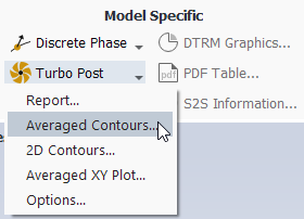
You can display contours using the Turbo Averaged Contours Dialog Box (Figure 14.32: The Turbo Averaged Contours Dialog Box).
![]() Results →
Model Specific → Turbo Post
→ Averaged Contours...
Results →
Model Specific → Turbo Post
→ Averaged Contours...
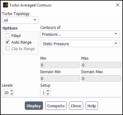
The basic steps for generating a turbo averaged contour plot are as follows:
Select All or a specific predefined turbomachinery topology from the Turbo Topology drop-down list.
Select the variable or function to be displayed in the Contours of drop-down list. First select the desired category in the upper list; you may then select a related quantity in the lower list. (See Turbomachinery-Specific Variables for a list of turbomachinery-specific variables, and see Field Function Definitions for an explanation of the variables in the list.)
Specify the number of contours in the Levels field. The maximum number of levels allowed is 100.
Click to display the specified contours in the active graphics window.
The resulting display will include the specified number of contours of the selected variable, with the magnitude on each one determined by equally incrementing between the values shown in the Min and Max fields.
Note that the Min and Max values displayed in the dialog box are the minimum and maximum averaged values. These limits will in general be different from the global Domain Min and Domain Max, which are also displayed for your reference (see Figure 14.32: The Turbo Averaged Contours Dialog Box).
The options mentioned in the procedure above include drawing color-filled contours (instead of line contours), specifying a range of values to be contoured, and storing the contour plot settings. These options are the same as those in the standard Contours Dialog Box. See Contour and Profile Plot Options for details about using them.
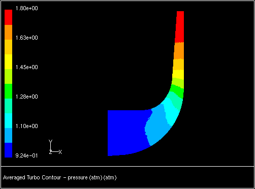
In postprocessing a turbomachinery solution, it is often desirable to display contours on surfaces of constant spanwise coordinate, and then project these contours onto a plane. This permits easier evaluation of the contours, especially for surfaces that are highly three-dimensional.
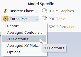
You can display contours using the Turbo 2D Contours Dialog Box (Figure 14.34: The Turbo 2D Contours Dialog Box).
![]() Results →
Model Specific → Turbo Post
→ 2D Contours...
Results →
Model Specific → Turbo Post
→ 2D Contours...
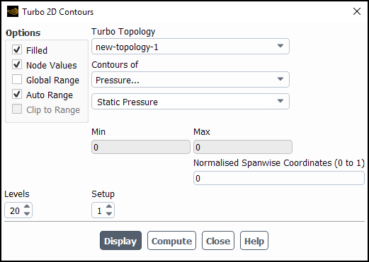
The basic steps for generating a turbo 2D contour plot are as follows:
Specify a specific predefined turbomachinery topology using the Turbo Topology drop-down list.
Enter a value for the Normalized Spanwise Coordinates (0 to 1) for the spanwise surface you want to create.
Select the variable or function to be displayed in the Contours of drop-down list.
First select the desired category in the upper list; you may then select a related quantity in the lower list. See Turbomachinery-Specific Variables for a list of turbomachinery-specific variables, and see Field Function Definitions for an explanation of the variables in the list.
Specify the number of contours in the Levels field. The maximum number of levels allowed is 100.
Click to display the specified contours in the active graphics window.
The resulting display will include the specified number of contours of the selected variable, with the magnitude on each one determined by equally incrementing between the values shown in the Min and Max fields.
Depending on the type of contour plot you want to display, select appropriate choice under Options. These options are the same as those in the standard Contours Dialog Box. See Contour and Profile Plot Options for details about using them.
When comparing numerical solutions of turbomachinery problems to experimental data, it is often useful to plot circumferentially averaged quantities in the spanwise and meridional directions. This section describes how to do this in Ansys Fluent.
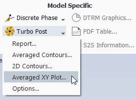
To create an XY plot of circumferentially averaged solution data, you will use the Turbo Averaged XY Plot Dialog Box (Figure 14.35: The Turbo Averaged XY Plot Dialog Box).
![]() Results →
Model Specific → Turbo Post
→ Averaged XY Plot...
Results →
Model Specific → Turbo Post
→ Averaged XY Plot...
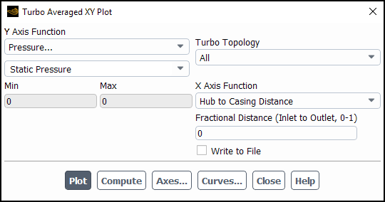
The procedure for generating a turbo averaged XY plot are as follows:
Select the variable or function to be plotted in the Y Axis Function drop-down list. First select the desired category in the upper list; you may then select a related quantity in the lower list. (See Turbomachinery-Specific Variables for a list of turbomachinery-specific variables, and see Field Function Definitions for an explanation of the variables in the list.)
Select All or a specific predefined turbomachinery topology from the Turbo Topology drop-down list.
Select the variable or function to be plotted in the X Axis Function drop-down list. The choices are Hub to Casing Distance and Meridional Distance.
Specify the desired value in the Fractional Distance field. The definition of the fractional distance depends on your selection of X Axis Function:
(optional) Modify the attributes of the axes or curves as described in Modifying Axis Attributes and Modifying Curve Attributes.
Click to generate the XY plot in the active graphics window.
Note that you can use any of the mouse buttons to annotate the XY plot (see Adding Text to the Graphics Window).
If you want to write the XY data to a file, follow these steps instead of Step 5 above:
Enable the Write to File option. The button changes to a Write... button.
In The Select File Dialog Box, specify a name for the plot file and save it.
In some cases, that is, isosurface creation, Ansys Fluent enables you to globally set the current turbomachinery topology for your model using the Turbo Options Dialog Box (Figure 14.36: The Turbo Options Dialog Box).
![]() Results → Model
Specific → Turbo Post
→ Options...
Results → Model
Specific → Turbo Post
→ Options...
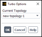
To set the current topology, select a topology from the Current Topology drop-down list and select .
An additional tool is available to calculate performance characteristics of a turbomachine. These characteristics are defined using Named Expressions and include efficiency, total pressure and total temperature ratios, as well as mass flow rates at the inlet and outlet.
You can define and evaluate performance characteristics for a turbomachine using the Turbo Performance dialog box (Figure 14.37: The Turbo Performance Dialog Box) accessed from:
![]() Domain → Turbomachinery
→
Domain → Turbomachinery
→
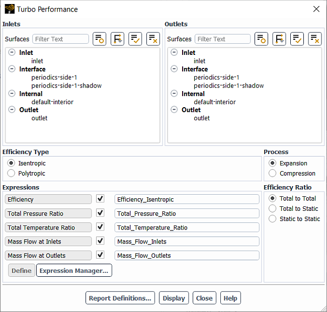
Select locations for the Inlets and Outlets using the corresponding surface lists. These lists are filtered to include only the surfaces of supported types.
Under Efficiency Type, select whether to compute the Isentropic or Polytropic efficiency.
Under Process, select whether to compute the performance characteristics for an Expansion or Compression process.
Under Efficiency Ratio, you can select which values are used when computing the turbomachine efficiency: Total to Total, Total to Static, or Static to Static.
You can define expressions for performance characteristics based on the dialog box input. Select the performance characteristics for which to define an expression. Optionally edit the default names (an integer number will be appended to each name automatically) and click Define to create expressions for each performance characteristic. All available expressions can be viewed and/or edited by clicking Expression Manager…. For more details, see Calculating Efficiency using Named Expressions, Calculating Total Pressure and Total Temperature Ratios using Named Expressions and Calculating Mass Flow Rates using Named Expressions.
Click Report Definitions… to open a dialog box which allows you to monitor, print, write, and/or plot the values of the expressions defined in the previous step. For more information, refer to Expression Report Definition.
Click Display to visualize the selected surfaces.
You can also access this tool by using the following console command and following the prompts:
/define/turbo-model/performance
You can compute the values of isentropic and polytropic efficiencies for a turbomachine using Named Expressions as shown in Figure 14.38: Expression Dialog Box with Efficiency Calculation.
![]() → User Defined → User
Defined → Named
Expressions → New...
→ User Defined → User
Defined → Named
Expressions → New...
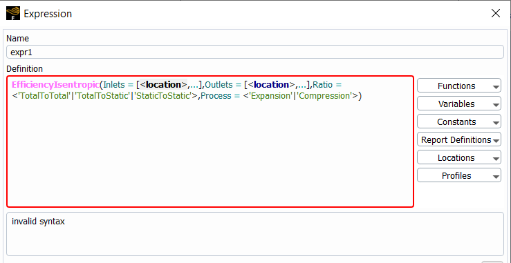
Functions for both efficiency types are listed under
Functions → Reduction as
EfficiencyIsentropic and
EfficiencyPolytropic.
Permeable boundaries of various types (for example, inlets, outlets, interfaces), as well as cut-planes and iso-surfaces, can be chosen as locations. Also, groups of surfaces for postprocessing is supported.
For the argument Inlets, you can select one or more locations
of mixed types. However, multiple locations will still be treated as the single-stream
inlet with properties averaged over all selected locations. This averaged inlet can be
considered as the starting point for efficiency calculation. Similarly, the end point will
be determined by locations selected for the argument Outlets.
Options for the argument Process(Expansion and Compression)
specify whether the flow expands or compresses when moving from the inlet to the outlet.
Options for the argument Ratio
(TotaltoTotal, TotaltoStatic and
StatictoStatic) determines the values used in computing the
efficiency.
Efficiency can be evaluated only for compressible flows of ideal gas, single-component real gas, and condensing water vapor (Wet Steam model).
Only the following locations are supported: Pressure Inlet, Pressure Outlet, Mass-Flow Inlet, Mass-Flow Outlet, Velocity Inlet, Pressure-far-field, Inlet Vent, Outlet Vent, Intake Fan, Exhaust Fan, Interior, Interface, Cut-plane, Iso-surface, Groups of listed surfaces.
Multiple inlet or outlet locations are reduced to a single stream with flow properties averaged over all selected.
After you have defined Turbo Topology (as described in Defining the Turbomachinery Topology), an additional option is available to compute efficiency using the Turbo Report dialog box as described in Generating Reports of Turbomachinery Data.
![]() → Results → Model
Specific → Turbo
Post → Report...
→ Results → Model
Specific → Turbo
Post → Report...

By default, the Turbo Report dialog box computes the Total to
Total values of isentropic and polytropic efficiencies assuming constant values of the
specific heat capacity Cp and heat capacity ratio γ. You can switch to the more
general equations which are implemented in the
EfficiencyIsentropic and
EfficiencyPolytropic functions, by using the following console
command:
/report/efficiency/use-in-turbo-report?
Note that for an ideal gas with constant Cp value, the two methods give nearly
identical results. However, for other cases, only the methods from the
EfficiencyIsentropic and
EfficiencyPolytropic functions are able to provide appropriate
efficiency values.
The Turbo Performance tool uses the
MassFlowAveAbs function to compute the values of total pressure
and total temperatures ratios. Named Expressions for these values are
defined as follows:
MassFlowAveAbs(Field,['location_1'])/MassFlowAveAbs(Field,['location_2'])
where the first argument Field is
TotalPressure or TotalTemperature. For
the Expansion process, the second argument
['location_1'] is the list of inlet zones and
['location_2'] is the list of outlet zones selected in the
dialog box. For the Compression process, the locations are reversed
with ['location_1'] being the list of outlet zones and
['location_2'] being the list of inlet zones selected in the
dialog box.
The MassFlowAveAbs function is listed under
Functions → Reduction in the
Expression dialog box. For more information on this and other
functions from the Named Expressions library, refer to Fluent Expressions Language.
The Turbo Performance tool uses the
MassFlowInt function to compute mass flow at inlets and
outlets. Named Expressions are defined as follows:
MassFlowInt(1, ['locations'])
The argument ['locations'] is the list of inlet or outlet
zones selected in the dialog box for the definition of the corresponding
expression.
The MassFlowInt function is listed under
Functions → Reduction in the
Expression dialog box. For more information on this and other
functions from the Named Expressions library, refer to Fluent Expressions Language.