51.19. Plots Task Page

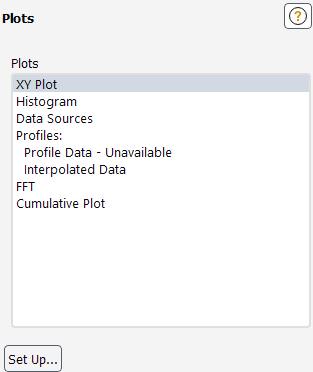
The Plots task page allows you to create plots (XY, histograms, profiles, and so on) of your computational results. See Displaying Graphics for more information.

Controls

Plots

contains a listing of the various plot types available in Ansys Fluent.

You can double-click an item in the Plots list to open the corresponding dialog box, or you can select the item in the list and click the Set Up... button.

XY Plot

selecting this item and clicking the Set Up... button opens the Solution XY Plot Dialog Box.

Histogram

selecting this item and clicking the Set Up... button opens the Histogram Dialog Box.

File

selecting this item and clicking the Set Up... button opens the Plot Data Sources Dialog Box.

Profiles

two types of profile plots are available:

Profile Data: selecting this item and clicking the Set Up... button opens the Plot Profile Data Dialog Box.
Interpolated Data: selecting this item and clicking the Set Up... button opens the Plot Interpolated Data Dialog Box.

FFT

selecting this item and clicking the Set Up... button opens the Fourier Transform Dialog Box.

Set Up...

displays the dialog box corresponding to the selected item in the Plots list.

For additional information, see the following sections:

51.19.1. Solution XY Plot Dialog Box

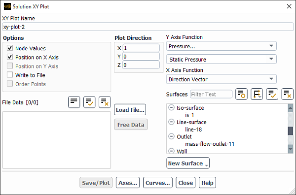
The Solution XY Plot dialog box allows you to display zone, surface and file data in an XY plot format. See Steps for Generating Solution XY Plots for details about the items below.

You can also access the Solution XY Plot dialog box through the Postprocessing ribbon tab.

Postprocessing → Plots → XY Plot → New...

Note:

The "global"/non-persistent form of graphics objects is hidden by default. If this interrupts your workflow, you can make them available by enabling the Expose legacy non-persistent graphics option in the Graphics branch of Preferences (accessed via File>Preferences...).
(When you click Edit... instead of New..., it opens the "global"/non-persistent version of the Solution XY Plot dialog box. This version of the dialog box does not have a Name field and it is not saved with the case file.
You are encouraged to use the persistent version that is accessed by clicking New....

Controls

XY Plot Name

is the name for a solution XY plot definition. You can specify a name or use the default name xy-plot-id. This control appears only for solution XY plot definitions.

Options

contains check buttons that control the presentation of node or cell-averaged values, the selection of axis functions, and the ability to write the plot data to a file.

Node Values: toggles the node averaging of the data presented in the plot. If the option is disabled, boundary face values are presented. See Choosing Node or Cell Values for details.
Position on X Axis, Position on Y Axis: set the -axis or -axis function to be the position. If one of these options is turned on, the other will automatically be turned off. You can turn both options off to generate a plot of one flow-field function vs. another, selecting the function for each axis using the X Axis Function and Y Axis Function drop-down lists.
Write to File: activates the file-writing option. When this option is selected, the Plot push button will change to Write.... Clicking on the Write... button will open the Select File dialog box (The Select File Dialog Box), in which you can specify a name and save a file containing the plot data. The format of this file is described in XY Plot File Format.
Order Points: specifies that plot data being saved to a file should be sorted in order of ascending axis value. This option is available only when the Write to File option is turned on.

Plot Direction

contains inputs for defining the plot direction.

If Direction Vector (the default) is selected in the X Axis Function or Y Axis Function drop-down list (whichever is the position axis), the inputs are the components of the direction vector. The position axis of the plot will have coordinate values that correspond to the dot product of the data coordinate vector with the plot direction vector. See Steps for Generating Solution XY Plots for details.

X: is the component in the direction.
Y: is the component in the direction.
Z: is the component in the direction.

If Curve Length is selected in the X Axis Function or Y Axis Function drop-down list (whichever is the position axis), the inputs are the direction along the length of the surface selected in the Surfaces list. See Steps for Generating Solution XY Plots for details.

Default: specifies the plot direction as the direction of increasing curve length.
Reverse: specifies the plot direction as the direction of decreasing curve length.
Show: displays the selected surface in the graphics window, marking the start of the surface with a blue dot and the end of the surface with a red dot. Ansys Fluent will also display arrows on the surface showing the direction in which the variable will be plotted.

Y Axis Function, X Axis Function

contain lists of solution variables that can be used for the or axis of the plot. If the Position on X Axis option is turned on, X Axis Function will become a single drop-down list, containing two options: Direction Vector (to plot the selected variable as a function of position along a specified direction vector) and Curve Length (to plot the selected variable as a function of position along the length of a specified curvilinear surface). See Steps for Generating Solution XY Plots for details.

Likewise, if Position on Y Axis is turned on, Y Axis Function will become a single drop-down list containing Direction Vector and Curve Length. If both Position on X Axis and Position on Y Axis are turned off, you can select field functions for both axes using the X Axis Function and Y Axis Function lists.

Note: When running the parallel version of Ansys Fluent, Curve Length is only supported when the curvilinear surface is contained within a single partition.

File Data

is a selectable list of the plot titles associated with the loaded external data files. You may choose any number of files for the data plot. The files are loaded using the Load File... push button. The format of these files is presented in XY Plot File Format. See Including External Data in the Solution XY Plot for details.

Load File...

opens the Select File dialog box (The Select File Dialog Box), in which you can select the plot file to be read. See Including External Data in the Solution XY Plot for details. After the external file is loaded, its plot title will be displayed in the File Data list.

Free Data

removes the files selected in the File Data list.

Surfaces

is a selectable list of surfaces in the solution domain. You may choose any number of surfaces for the data plot.

New Surface

is a drop-down list button that contains a list of surface options:

Point: opens the Point Surface Dialog Box.
Line/Rake: opens the Line/Rake Surface Dialog Box.
Plane: opens the Plane Surface Dialog Box.
Quadric: opens the Quadric Surface Dialog Box.
Iso-Surface: opens the Iso-Surface Dialog Box.
Iso-Clip: opens the Iso-Clip Dialog Box.
Structural Point: opens the Structural Point Surface Dialog Box.

Plot

plots the specified surface and/or file data in the active graphics window using the current axis and curve attributes. If the Write to File option is turned on, this button becomes the Write... button.

Write...

opens the Select File dialog box (The Select File Dialog Box), in which you can save the plot data to a file. This button replaces the Plot button when the Write to File option is turned on.

Axes...

opens the Axes Dialog Box, which allows you to customize the plot axes.

Curves...

opens the Curves Dialog Box, which allows you to customize the curves used in the XY plot.

Save/Plot

plots the specified surface and/or file data in the active graphics window using the current axis and curve attributes and saves the XY plot definition. This button appears only for solution XY plot definitions and replaces the Plot button.

51.19.2. Histogram Dialog Box

The Histogram dialog box allows you to create histograms of selected geometric or physical data. See Steps for Generating Histogram Plots for details about the items below.

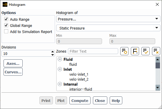
Controls

Options

contains the check buttons for current histogram options.

Auto Range: toggles the ability to specify the minimum and maximum range of scalar values in the histogram print or plot. If the option is not active, the Min and Max fields are editable, and you may specify the desired range. If the option is active, the range is defined by the minimum and maximum values in the computational domain.
Global Range: toggles the ability to specify the minimum and maximum values on the range of values on the selected surfaces, rather than in the entire domain.
Add to Simulation Report: toggles the ability to add the histogram and its data to your simulation report.

Divisions

sets the number of data intervals that will exist in the histogram.

Zone Types

contains a list of available face or cell zone types.

Axes...

opens the Axes Dialog Box, which allows you to customize the plot axes.

Curves...

opens the Curves Dialog Box, which allows you to customize the curves used in the histogram plot.

Histogram of

contains a list of scalar quantities that can be used in the histogram.

Min

displays or allows definition of the minimum value of the selected scalar quantity used in the histogram.

Max

displays or allows definition of the maximum value of the selected scalar quantity used in the histogram.

Zones

contains a list of available face or cell zones.

Print

displays the histogram interval.

Plot

displays a plot of the percentage of the total number of cells versus the scalar quantity in the active graphics window.

Add To Report

adds the histogram and its data to the simulation report (when the Add to Simulation Report option is enabled).

Compute

computes the minimum and maximum cell values of the selected scalar quantity. The values are displayed in Min and Max.

51.19.3. Plot Data Sources Dialog Box

The Plot Data Sources dialog box allows you display data read from one or more files (in an abscissa/ordinate plot form) and combine them with data from XY plot objects and report plots. The format of the plot file is described in XY Plot File Format. See Steps for Generating XY Plots of Data from Multiple Sources for details about the items below.

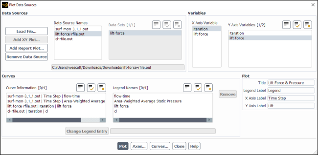
Controls

Data Sources

contains operations and information related to the selected files/plots.

Load file...: opens the Select File dialog box, where you can select the file(s) you want to plot.
Add XY Plot...: opens the Select Plots dialog box, where you can select the plot(s) you want to include.
Add Report Plot...: opens the Select Plots dialog box, where you can select the report plot(s) you want to include.
Remove Data Source: removes the selected data source from the Data Source Names list. This also removes any curves associated with that file.
Data Source Names: lists the files and plots that you have loaded.
Data Sets: lists the available data sets for files and plots (typically .xy) that contain two columns monitoring the same value at different locations. You can select which data sets you want to plot by selecting/de-selecting the listed items.

Variables

lists X and Y variables for the selected file.

X Axis Variable: lists the variables that you can select for the X axis. The highlighted X variable will be added to the Curve Information list in coordination with the selected Y Axis Variables. Changing the selected X Axis Variable updates all the related curves shown in the Curve Information list.

Y Axis Variables: lists the variables that you can select for the Y axis. The highlighted Y variables will be added to the Curve Information list in coordination with the selected X Axis Variable. Changing the selected Y Axis Variables updates how many curves are shown in the Curve Information list.

Curves

lists what items will be plotted and how they will be labeled in the legend.

Curve Information

lists the curves that will be plotted.

Information about each curve is shown in the following order:

The name of the file where the data originated.
[2 column file (typically .xy) only] The location on the model where the data originated.
X Variable.
Y Variable.

Legend Names

lists the name for each curve that will be listed in the legend when the plot is displayed in the graphics window. (see Change Legend Entry to learn how to change the legend name for a curve).

Remove

removes the selected curve from the Curve Information list.

Change Legend Entry

allows you to change the name that will appear in the plot legend in the graphics window for a particular curve.

To use:

Select a name in the Legend Names list.
Enter the new name in the text entry box to the right of the Change Legend Entry button.
Click Change Legend Entry.

Plot

contains text entry boxes for the various plot labels.

Title: lets you enter a title for the plot.
Legend Label: lets you enter a title for the legend.
X Axis Label: lets you label the X axis.
Y Axis Label: lets you label the Y axis.

Plot (button): click Plot to plot the data listed in the Curve Information list.

Axes... (button): opens the Axes dialog box, which allows you to customize the plot axes.

Curves... (button): opens the Curves dialog box, which allows you to customize the curves used in the XY plot.

51.19.4. Plot Profile Data Dialog Box

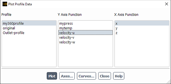
The Plot Profile Data dialog box allows you to display an XY plot of the original data points of a boundary profile before it is interpolated onto the cell faces of a boundary. See Steps for Generating Plots of Profile Data for details about the items below.

Controls

Profile: contains a selectable list of available profiles. When a profile is selected its available fields are displayed under Y Axis Function.
Y Axis Function: contains a selectable list of the fields available in the selected profile that can be used for the axis of the plot.
X Axis Function: contains a selectable list of the variables that can be used for the axis of the plot.
Plot: displays an XY plot of the data points from the selected profile.
Axes...: opens the Axes Dialog Box, which allows you to customize the plot axes.
Curves...: opens the Curves Dialog Box, which allows you to customize the curves used in the XY plot.

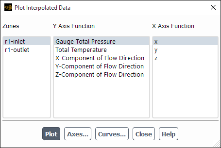
51.19.5. Plot Interpolated Data Dialog Box

The Plot Interpolated Data dialog box allows you to display an XY plot of the values assigned to the cell faces when a profile file has been interpolated on a boundary. See Steps for Generating Plots of Interpolated Profile Data for details about the items below.

Controls

Zones: contains a selectable list of the zones for which a profile field has been set as one or more of the parameters are displayed under Y Axis Function.
Y Axis Function: contains a selectable list of the profile-related parameters in the selected zone that can be used for the axis of the plot. The name of the parameter will be the same as that of the drop-down list in the boundary condition dialog box from which the profile field was selected.
X Axis Function: contains a selectable list of the geometry variables that can be used for the axis of the plot.
Plot: displays an XY plot of the cell face values (as interpolated from the data points of the profile file) of the selected zone.
Axes...: opens the Axes Dialog Box, which allows you to customize the plot axes.
Curves...: opens the Curves Dialog Box, which allows you to customize the curves used in the XY plot.

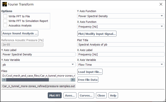
51.19.6. Fourier Transform Dialog Box

The Fourier Transform dialog box allows you to analyze your time dependent data using the Fast Fourier Transform (FFT) algorithm. See Fast Fourier Transform (FFT) Postprocessing for details about the items below.

Controls

Options

lets you write the FFT data to a file or display the FFT data in a graphics window.

Write FFT to File: allows you to write out the FFT data directly to a file. When selected, the Plot FFT... buttons becomes the Write FFT... button.
Acoustics Analysis: enables the acoustics-relevant spectrum options (sound pressure level spectra and frequency band charts), and specifies that the overall sound pressure level is calculated and displayed in the console when you plot or write the FFT data. All dB-measured quantities are based on the Reference Acoustic Pressure.

Ansys Sound Analysis...

opens the Ansys Sound Analysis Dialog Box.

Process Options

contains options to analyze signal data.

Process Receiver: allows you to analyze receiver data stored in memory.
Process File Data: allows you to analyze signal data from an existing input file.

Y Axis Function

contains a list from which you can select the function for the axis.

X Axis Function

contains a list from which you can select the function for the axis.

Receiver

contains a list of receivers from which you can select when the Process Receiver option is enabled.

Plot/Modify Input Signal...

opens the Plot/Modify Input Signal Dialog Box, which you can use to plot the input signal, as well as customize the data set and define spectrum smoothing in preparation for applying the FFT algorithm.

Reference Acoustic Pressure

allows you to specify the reference acoustic pressure (for example, in Equation 40–15) used to calculate the dB-measured quantities when the Acoustics Analysis option is enabled.

Plot Title

lets you create a new title or edit the original title for the FFT plot. By default, Ansys Fluent adds the string "Spectral Analysis of" to the title originally applied to the input signal plot.

Y Axis Label

allows you to create a new axis label or edit the original axis label. By default, the Y Axis Label corresponds to the selection in the Y Axis Function drop-down list.

X Axis Label

allows you to create a new axis label or edit the original axis label. By default, the X Axis Label corresponds to the selection in the X Axis Function drop-down list.

Y Axis Variable

if your input report file contains multiple report definitions, this allows you to specify the axis variable.

X Axis Variable

if your input report file contains multiple report definitions, this allows you to specify the axis variable.

Files

lists the loaded input signal data files.

Load Input File...

loads an input signal data file into Ansys Fluent for FFT analysis. The input file is listed under Files.

Free File Data

removes data from FFT analysis once the input signal data file is selected in the Files list.

Plot FFT

displays the FFT data in a graphic window and, if Acoustics Analysis is enabled, calculates the overall sound pressure level in dB (based on the Reference Acoustic Pressure) and displays it in the console. If the Write FFT to File option is selected, then this button becomes the Write FFT button, which opens a file selection dialog box so that you write the FFT data to a file.

Write FFT

opens The Select File Dialog Box in which you can specify a name and save the FFT data to a file. If Acoustics Analysis is enabled, the overall sound pressure level will be calculated in dB (based on the Reference Acoustic Pressure) and displayed in the console at this time. If the Write FFT to File option is selected, then the Plot FFT button changes to the Write FFT button.

Axes...

opens the Axes Dialog Box, which allows you to customize the plot axes.

Curves...

opens the Curves Dialog Box, which allows you to customize the curves used in the plot.

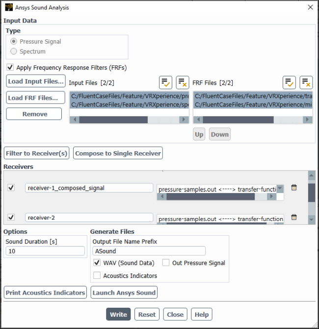
51.19.7. Ansys Sound Analysis Dialog Box

Refer to Performing an Ansys Sound Analysis for additional information on this dialog box.

Controls

Input Data

Pressure Signal: specifies that the input file you select is an acoustic pressure file (two column file of time vs. pressure).
Spectrum: specifies that the input file you select is an FFT output file (two column file of frequency vs. power spectral density).

Apply Frequency Response Filters (FRFs)

allows you to load a frequency response filter (FRF) file.

Load Input Files...

allows you to read in either a pressure data or spectrum input file.

Load FRF Files...

allows you to read in frequency response filter files.

Remove

removes the selected file from the Input Files and FRF Files lists.

Input Files

lists the loaded input pressure signal or spectrum files.

FRF Files

lists the loaded frequency response filter (FRF) files.

Up

moves the selected FRF file up in the list.

Down

moves the selected FRF file down in the list.

Filter to Receiver(s)

adds one or more receivers (based on the number of selected files) that are mapped with one input file and one frequency response filter file per receiver to the Receivers list. For example, you could have 3 input files and 3 FRF files selected and this would result in 3 new receivers. You could also have 1 input file selected and 3 FRF files selected, which would also result in 3 new receivers.

Compose to Single Receiver

combines the selected input files and corresponding FRF files into a single receiver that gets added to the Receivers list.

Receivers

lists the defined receivers and their comprising input and FRF files, with arrows indicating how they correspond.

Active: indicates whether the receiver is active. That is, whether or not the receiver will be included or evaluated when you click any of the following buttons: Print Acoustic Indicators, Launch Ansys Sound, Write.
Name: displays the (editable) name of each defined receiver.
Input Files <---> FRF Files: displays the input and FRF files included within a receiver. The arrow indicates which input file is modified by which FRF file.

Options

Sound Duration: specifies the length of the sound clip for saving a WAV file.

Generate Files

Output File Name Prefix: specifies the name (aside from the extension) for any files saved when you click Write.
WAV (Sound Data): specifies that a WAV sound file will be written when you click Write.
Out Pressure Signal: specifies that a pressure signal file will be written when you click Write.
Acoustic Indicators: specifies that a file containing the computed acoustic indicators will be written when you click Write.

Print Acoustic Indicators

computes the acoustic indicators for the selected files and prints them to the console.

Launch Ansys Sound

launches Ansys Sound and loads the defined receivers.

Write

computes the acoustic indicators for the selected files and prints them to the console.

Reset

clears all settings and default changes from the dialog box.

51.19.8. Cumulative Plot Dialog Box

The Cumulative Plot dialog box allows you to analyze the development of force, moments, or coefficients for your model in the any desired location or direction. See Cumulative Force, Moment, and Coefficients Plots for details about the items below.

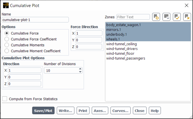
Controls

Name

name of the cumulative plot object.

Options

lets you select which type of plot to display.

Cumulative Force: displays the force development for the specified direction and walls.
Cumulative Force Coefficient: displays the force coefficient development for the specified direction and walls.
Cumulative Moments: displays the moment development for the specified direction and walls.
Cumulative Moment Coefficient: displays the moment coefficient development for the specified direction and walls.

Cumulative Plot Options

contains options to specify the direction and number of divisions where Fluent will calculate and plot the selected variable.

Direction: allows you to specify the direction along which the cumulative force or moments will be computed.
Number of Divisions: specifies the number of slices across the selected wall zones where the force or moments will be evaluated for the resulting cumulative plot. The planes will be created perpendicular to the Direction.

Compute from Force Statistics

use averaged values computed from force statistics instead of the default instantaneous values.

Force Direction

(Cumulative Force and Cumulative Force Coefficient only) allows you to specify the force component direction.

Moment Center

(Cumulative Moments and Cumulative Moment Coefficient only) allows you to specify the coordinates of the moment center.

Moment Axis

(Cumulative Moments and Cumulative Moment Coefficient only) allows you to specify the coordinates of the moment axis.

Zones

lists the zones that you can select for the cumulative plot.

Save/Plot

saves the cumulative plot object and plots the cumulative force, force coefficient, moments, or moment coefficient.

Write...

opens The Select File Dialog Box, allowing you to save the plot data to a file.

Print

prints the value of the force or moment at each division to the console.

Axes...

opens the Axes Dialog Box, which allows you to customize the plot axes.

Curves...

opens the Curves Dialog Box, which allows you to customize the curves used in the plot.

51.19.9. Plot/Modify Input Signal Dialog Box

The Plot/Modify Input Signal dialog box allows you to plot the input signal, as well as customize the data set and define spectrum smoothing in preparation for applying the FFT algorithm. It is opened from the Fourier Transform Dialog Box. See Using the FFT Utility for details about the items below.

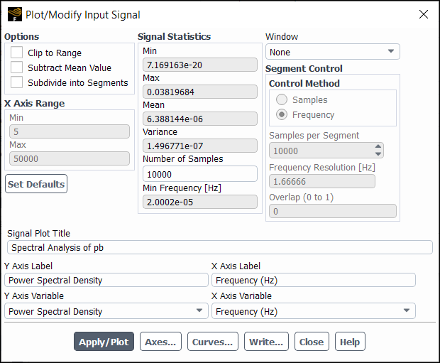
Controls

Options

allows you to process some or all of the input signal data.

Clip to Range: allows you to analyze a portion of the input signal by specifying data range.
Subtract Mean Value: reduces y axis quantities by the mean value of the relevant signal property.
Subdivide into Segments: enables / disables spectrum smoothing, which can suppress spurious amplitude fluctuations in the Fourier spectrum by splitting the input signal into multiple overlapping segments, so that Ansys Fluent can apply the FFT algorithm on each segment and then average the resulting spectra. The spectrum smoothing is controlled by the settings in the Segment Control group box. See Customizing the Input and Defining the Spectrum Smoothing for further details.

Signal Statistics

displays signal information.

Min: displays the minimum value for the input signal.
Max: displays the maximum value for the input signal.
Mean: displays the average value for the input signal.
Variance: displays the variance for the input signal.
Number of Samples: displays the total number of samples in the input signal data set.
Min Frequency: displays the finest possible frequency resolution for the input signal.

X Axis Range

allows for a portion of the input signal to be analyzed when the Process the whole data option is turned off.

Min: specifies a minimum value for the axis.
Max: specifies a maximum value for the axis.

Set Defaults

resets the axis minimum and maximum values to their original value and turns on the Process the whole data option.

Signal Plot Title

lets you create a new title or edit the original title for the input signal plot. By default, the Signal Plot Title corresponds with the title originally applied to the input signal plot.

Y Axis Label

allows you to create a new axis label or edit the original axis label. By default, the Y Axis Label corresponds with the axis label originally applied to the input signal plot.

X Axis Label

allows you to create a new axis label or edit the original axis label. By default, the X Axis Label corresponds with the axis label originally applied to the input signal plot.

Y Axis Variable

if your input report file contains multiple report definitions, this allows you to specify the axis variable.

X Axis Variable

if your input report file contains multiple report definitions, this allows you to specify the axis variable.

Window

lets you specify a windowing technique to remove discontinuities in the FFT calculation.

None: applies no windowing technique. This is the default setting.
Hamming: applies the Hamming technique.
Hanning: applies the Hanning technique.
Bartlett: applies the Bartlett technique.
Blackman: applies the Blackman technique.

Segment Control

provides settings that control the spectrum smoothing when Subdivide into Segments is enabled.

Control Method

allows you to specify how you want to define the segment size from the following:

Samples: bases the segment size on the Samples per Segment.
Frequency: bases the segment size on the Frequency Resolution in Hertz units.

Samples per Segment

defines the number of samples in each segment when Samples is selected from the Control Method list.

Frequency Resolution

defines the desired frequency resolution in Hertz units when Frequency is selected from the Control Method list.

Overlap

ranges from 0 to 1 and defines how much adjacent segments overlap. This setting is applicable regardless of which Control Method you select.

Apply/Plot

applies any changes you have made in the dialog box and displays the input signal data in a graphics window.

Axes...

opens the Axes Dialog Box, which allows you to customize the plot axes.

Curves...

opens the Curves Dialog Box, which allows you to customize the curves used in the plot.

Write...

opens The Select File Dialog Box, in which you can save the signals to a file.

51.19.10. Axes Dialog Box

The Axes dialog box allows you to independently control the characteristics of the ordinate and abscissa on an XY plot or histogram. You can change the titles, scale, range, number format, and major and minor rules visibility and appearance. Note that the title following Axes in the dialog box indicates which plot environment you are changing. You can set different parameters for each type of plot that Ansys Fluent can generate. See Using the Axes Dialog Box for details about the items below.

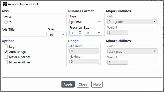
Controls

Axis

contains check buttons that allow you to set abscissa (-axis) or ordinate (-axis) characteristics.

X: allows you to specify the abscissa characteristics.
Y: allows you to specify the ordinate characteristics.

Axis Title

defines the character string that will label the active axis (the one selected in Axis) in the display.

Size

specifies the font size of the Axis Title.

Options

contains check buttons that (de)activate scale, range, major rules, and minor rules.

Log: toggles logarithmic scaling of the active axis. By default, decimal scaling is used.
Auto Range: toggles automatic computation of the range of the active axis. If you deactivate this option, you may input the Minimum and Maximum values in the Range box.
Major Rules: toggles the display of major rules on the active axis. Major rules are the horizontal or vertical lines that mark the primary data divisions and span the whole plot window to produce a "grid."
Minor Rules: toggles the display of minor rules on the active axis. Minor rules are the horizontal or vertical lines that mark the secondary data divisions and span the whole plot window to produce a "grid."

Number Format

contains controls for changing the format of the data labels on the active axis. Data labels are the character strings used to define the primary data divisions on the axes.

Type

sets the form of the data labels. You may select from a drop-down list of options, including the following:

general: displays the real value with either float or exponential form based on the size of the number and the defined Precision.
float: displays the real value with an integral and fractional part (for example, 1.0000), where the number of digits in the fractional part is determined by Precision.
exponential: displays the real value with a mantissa and exponent (for example, 1.0e-02), where the number of digits in the fractional part of the mantissa is determined by Precision.

Precision

defines the number of fractional digits displayed in the data labels.

Size

specifies the size of the font used for the data labels.

Range

contains the range or extents of the active axis. To set the range manually, you must turn off Auto Range. Otherwise the extents are computed automatically.

Minimum: sets the minimum data value for the active axis.
Maximum: sets the maximum data value for the active axis.

Major Rules

contains controls for modifying the appearance of the major rules. To use these controls you must activate Major Rules in the Options list.

Color: sets the color of the major rules from a drop-down list with numerous color selections.
Weight: sets the line thickness of the major rule. A line of weight 1.0 is normally 1 pixel wide. A weight of 2.0 would make the line twice as thick (2 pixels wide).

Minor Rules

contains controls for modifying the appearance of the minor rules. To use these controls you must activate Minor Rules in the Options list.

Color: sets the color of the minor rules from a drop-down list with numerous color selections.
Weight: sets the line thickness of the minor rule. A line of weight 1.0 is 1 pixel wide. A weight of 2.0 would make the line twice as thick (2 pixels wide).

51.19.11. Curves Dialog Box

The Curves dialog box allows you to modify the appearance of the lines and markers used in XY plots. Note that the title following Curves in the dialog box indicates which plot environment you are changing. You can set different parameters for each type of plot that Ansys Fluent can generate. See Using the Curves Dialog Box for details about the items below.

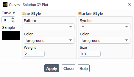
Controls

Curve #

defines the active curve number. The present and future marker and line styles apply to the defined curve number. The curves are numbered sequentially, starting from 0. For example, if you were plotting flow-field values on two zones, the first zone would be curve 0, and the second, curve 1. If the plot contains only one curve, the Curve # is set to 0 and is not editable.

Sample

displays a single marker and line with the current style attributes.

Line Style

contains controls for modifying the appearance of the active curve.

Pattern: sets the pattern of the active curve. A drop-down list allows you to set the line pattern. Except for center and phantom lines, the list displays examples of the pattern choices. A center line alternates a very long dash and a short dash and a phantom line alternates a very long dash and a double short dash.
Color: sets the color of the active curve. A drop-down list allows you to select from a list of color names.
Weight: sets the thickness of the active curve. A line weight of 1.0 is normally 1 pixel wide. Therefore, a weight of 2.0 would make the line twice as thick (2 pixels wide).

Marker Style

contains controls for modifying the appearance of the active curve’s marker.

Symbol: sets the symbol used to mark data. You can select the symbol from a drop-down list that contains all the symbol choices. The Sample box will allow you to experiment with various markers. For example, in plotting pressure-coefficient data on the upper and lower surfaces of an airfoil, the symbol /*\ (filled-in upward-pointing triangle) could be used for the marker representing the upper surface data, and the symbol \*/ (filled-in downward-pointing triangle) could be used for the marker representing the lower surface data.
Color: sets the color of the marker on the active line number. A drop-down list allows you to select from a list of color names.
Size: sets the size of the data marker. A symbol of size 1.0 is 3.0% of the height of the display screen, except for the "." symbol, which is always one pixel.