


For additional information, see the following sections:
The pressure-velocity coupling scheme controls the manner in which pressure and velocity are updated when the pressure-based solver is used. The scheme can be either segregated (pressure and velocity are updated sequentially) or coupled (pressure and velocity are updated simultaneously).
Ansys Fluent provides the following segregated types of algorithms:
SIMPLE
SIMPLEC
PISO
Fractional Step (FSM) (time-dependent flows with Non-Iterative Time Advancement (NITA) only)
In general, segregated methods are faster per iteration, while the coupled algorithm usually requires fewer iterations to converge. For this reason, the coupled solver is usually recommended for steady-state simulations. For transient simulations, the coupled solver has the best robustness properties, especially for large time step sizes, but SIMPLEC, PISO, or NITA may give faster overall solution times for small time step sizes.
Note: Steady-state and transient simulations differ in their default selection for the pressure-velocity coupling scheme. If you select a scheme, it will not necessarily be retained if you then switch between a steady and transient calculation.
The following mechanisms are available to under-relax the equations:
Pseudo time method (not available for the transient coupled solver)
Courant number (coupled solver only)
The coupled solver with a pseudo time method selected is the default for cases with the following settings:
Steady-state
Single-phase
No battery or fuel cell model
No solidification and melting model
Limitations and controls for the pseudo time method are described in Performing Calculations with a Pseudo Time Method. The most important (and typically the only) control you need to adjust in practice is the Pseudo Time Step Size for the coupled solver or the Pseudo Time Courant Number for the segregated solver, as described in Pseudo Time Settings for the Calculation.
Important: Pressure-velocity coupling is relevant only for the pressure-based solver.
In Ansys Fluent, both the standard SIMPLE algorithm and the SIMPLEC (SIMPLE-Consistent) algorithm are available. SIMPLE is the default for transient simulations, but many problems will benefit from using SIMPLEC, particularly because of the increased under-relaxation that can be applied, as described below.
For relatively uncomplicated problems (laminar flows with no additional models enabled) in which convergence is limited by the pressure-velocity coupling, you can often obtain a converged solution more quickly using SIMPLEC. With SIMPLEC, the pressure-correction under-relaxation factor is generally set to 1.0, which aids in convergence speed-up. In some problems, however, increasing the pressure-correction under-relaxation to 1.0 can lead to instability due to high mesh skewness. For such cases, you will need to use one or more skewness correction iterations, use a slightly more conservative under-relaxation value (up to 0.7), or use the SIMPLE algorithm. For complicated flows involving turbulence and/or additional physical models, SIMPLEC will improve convergence only if it is being limited by the pressure-velocity coupling. Often it will be one of the additional modeling parameters that limits convergence; in this case, SIMPLE and SIMPLEC will give similar convergence rates.
The PISO algorithm (see PISO in the Theory Guide) with neighbor correction is highly recommended for all transient flow calculations, especially when you want to use a large time step size. (For problems that use the LES turbulence model, which usually requires a small time step size, using PISO may result in an increased computational expense, so SIMPLE or SIMPLEC should be considered instead.) PISO can maintain a stable calculation with a larger time step size and an under-relaxation factor of 1.0 for both momentum and pressure. For steady-state problems, PISO with neighbor correction does not provide any noticeable advantage over SIMPLE or SIMPLEC with optimal under-relaxation factors.
PISO with skewness correction is recommended for both steady-state and transient calculations on meshes with a high degree of distortion.
When you use PISO neighbor correction, under-relaxation factors of 1.0 or near 1.0 are recommended for all equations. If you use just the PISO skewness correction for highly-distorted meshes (without neighbor correction), set the under-relaxation factors for momentum and pressure so that they sum to 1 (for example, 0.3 for pressure and 0.7 for momentum). If you use both PISO skewness correction and neighbor correction, follow the under-relaxation recommendations for PISO neighbor correction, above.
For most problems, it is not necessary to disable the default coupling between neighbor and skewness corrections. For highly distorted meshes, however, disabling the default coupling between neighbor and skewness corrections is recommended.
The Fractional Step method (FSM), described in Fractional-Step Method (FSM) in the Theory Guide, is available when you choose to use the NITA scheme (that is, the Non-Iterative Time Advancement option in the Solution Methods task page). With the NITA scheme, the FSM is slightly less computationally expensive compared to the PISO algorithm. Whether you select FSM or PISO depends on the application. For some problems (for example, simulations that use VOF), FSM could be less stable than PISO.
In most cases, the default values for the solution methods are enough to set a robust convergence of the internal pressure correction sub-iterations due to skewness. Only very complex problems (for example, moving deforming meshes, sliding interfaces, or the VOF model) could require a reduction of relaxation for pressure up to a value of 0.7 or 0.8.
Selecting Coupled from the Pressure-Velocity Coupling drop-down list indicates that you are using the pressure-based coupled algorithm, described in Coupled Algorithm in the Theory Guide. This solver offers some advantages over the pressure-based segregated algorithm. The pressure-based coupled algorithm obtains a more robust and efficient single phase implementation for steady-state flows. It is not available for cases using the Non-Iterative Time Advancement option (NITA).
Note: In some cases using porous jump boundary conditions, the Coupled scheme may suffer from convergence issues that do not respond to changes in the coupled solver settings. This behavior depends on the specific flow configuration and porous jump boundary condition values. If convergence instability is observed in cases using porous jump boundary conditions and the scheme, it is recommended that you change the pressure-velocity coupling to one of the segregated schemes.
You can specify the pressure-velocity coupling method in the Solution Methods Task Page (Figure 36.4: The Solution Methods Task Page for a Pressure-Based Segregated Algorithm).
![]() Solution →
Solution → ![]() Methods
Methods
Choose SIMPLE, SIMPLEC, PISO, Fractional Step, or Coupled in the Pressure-Velocity Coupling drop-down list.
If you choose PISO, the task page will expand to show
the additional parameters for pressure-velocity coupling. By default, the number
of iterations for Skewness Correction and
Neighbor Correction are set to 1.
If you want to use only Skewness Correction, then set the
number of iterations for Neighbor Correction to
0. Likewise, if you want to use only Neighbor
Correction, then set the number of iterations for Skewness
Correction to 0. For most problems, you do
not need to change the default iteration values. By default, the
Skewness-Neighbor Coupling option is enabled to allow for a
more economical, but a less robust variation of the PISO algorithm. For further
details, see Neighbor Correction, Skewness Correction, and Skewness - Neighbor Coupling in the Fluent Theory Guide.
If you choose SIMPLEC under Pressure-Velocity
Coupling, you can also increase the number of iterations for the
Skewness Correction from the default value of
0. For further details, see Skewness Correction in the Fluent Theory Guide.
When a segregated solver is selected, you can use the following text command to enable an enhanced formulation for the skewness correction that computes the pressure-correction gradient. It is only used during the simulation when SIMPLEC or PISO is selected with one or more active Skewness Correction iterations. In a mesh with very skewed elements, the enhanced formulation should improve solver robustness—that is, avoid stalled convergence or divergence—when compared to the default skewness correction formulation. In the rare case where it decreases stability, you can attempt to remedy it by lowering the under-relaxation factor and (for PISO) disabling the Skewness-Neighbor Coupling option. Note that the use of either default or enhanced skewness correction formulation does not affect the accuracy of a converged simulation.
solve → set
→ advanced →
skewness-correction-enhanced
If you choose SIMPLE, SIMPLEC, or
PISO and select Local Time Step from
the Pseudo Time Method drop-down list, you will have to
specify the Pseudo Time Courant Number in the
Solution Controls task page, which is set at
5 by default. For more information, refer to Local Time Step Method in the Theory Guide.
If you choose Coupled for a transient case or select
Off from the Pseudo Time Method
drop-down list for a steady case, you will have to specify the Flow
Courant Number in the Solution Controls task
page, which is set at 200 by default. You will also
specify the Explicit Relaxation Factors for
Momentum and Pressure, which are set
at 0.5 by default. For more information about these
options, refer to Pressure-Velocity Coupling and Steady-State Iterative Algorithm in the
Theory Guide.
For cases with very skewed meshes, the run can be stabilized by further
reduction of the explicit relaxation factor to 0.25. If
Ansys Fluent immediately diverges in the AMG solver, then the CFL number is too
high and should be reduced. Reducing the CFL number below
10 is not recommended since it would be better to use
the segregated algorithm for the pressure-velocity coupling.
In most transient cases, the CFL number should be set to a large value such as 107 and explicit relaxation factors to 1.0.
If you choose Coupled and have Global Time Step selected from the Pseudo Time Method drop-down list, you will set the Pseudo Time Explicit Relaxation Factors in the Solution Controls task page, as described in Global Time Step Method Settings.
The method for calculating the mass flux is defined using the Flux Type drop-down list in the Solution Methods task page.
![]() Solution →
Solution → ![]() Methods
Methods
For the pressure-based solver, Fluent offers two formulations for the mass flux computation:
Rhie-Chow: momentum based
This flux option follows a momentum-coefficient-weighted high-order velocity interpolation with a Rhie-Chow correction for the pressure gradient difference.
Rhie-Chow: distance based
This flux option applies a distance-weighted high-order velocity interpolation with a Rhie-Chow correction for the pressure gradient difference.
By default, the Auto Select option is enabled next to the Flux Type list so that Fluent automatically selects the most robust flux formulation based on the flow models and mesh attributes. The Rhie-Chow: momentum based option is selected for most cases. The Rhie-Chow: distance based option is automatically selected only for the following combination: a transient simulation that uses a Scale-Resolving Simulation (SRS) model (see Scale-Resolving Simulation (SRS) Models), a compressible fluid, and an adapted mesh. In this context, a mesh is considered to be adapted if you have manually adapted the mesh (even if you subsequently coarsened the mesh), you have defined automatic adaption criteria prior to starting the calculation, and/or it is a hexcore, poly-hexcore, or CutCell mesh (see Generating the Hexcore Mesh, Generating Poly-Hexcore Meshes, or Generating the CutCell Mesh, respectively) that has a hanging node as the result of hex refinement.
Note: The following statements describe the behavior of the automatic selection of the mass flux formulation after a time step has been calculated:
The automatic flux type selection will not change if you then adapt the mesh or define an automatic adaption criterion. In such circumstances it is generally preferable to continue with the same flux type rather than to risk a jump in the residuals.
The automatic flux type selection may change if you make a change in the temporal discretization (steady vs. transient), material property (compressible vs. incompressible), and/or turbulence model (scale-resolving vs. non-scale-resolving); you will be notified of such a change by an Information dialog box and a note in the console.
If you want greater control over the choice of mass flux formulation, you can disable the Auto Select option and then manually select your preferred flux formulation from the Flux Type drop-down list.
For further details about the Flux Type options, see Discretization of the Continuity Equation in the Fluent Theory Guide.
Note: For multiphase models other than the wet steam model, the Flux Type list is not available and the Rhie-Chow: momentum based flux option is used.
The pressure-based solver uses under-relaxation of equations to control the update of computed variables at each iteration (as described in Under-Relaxation of Equations in the Theory Guide). This means that all equations solved using the pressure-based solver, including the non-coupled equations solved by the density-based solver (turbulence and other scalars, as discussed in Density-Based Solver in the Theory Guide), will have under-relaxation factors associated with them.
In Ansys Fluent, the default under-relaxation parameters for all variables are set to values that are near optimal for the largest possible number of cases. These values are suitable for many problems, but for some particularly nonlinear problems (for example, some turbulent flows or high-Rayleigh-number natural-convection problems) it is prudent to reduce the under-relaxation factors initially.
It is good practice to begin a calculation using the default under-relaxation factors. If the residuals continue to increase after the first 4 or 5 iterations, you should reduce the under-relaxation factors.
Occasionally, you may make changes in the under-relaxation factors and resume your calculation, only to find that the residuals begin to increase. This often results from increasing the under-relaxation factors too much. A cautious approach is to save a data file before making any changes to the under-relaxation factors, and to give the solution algorithm a few iterations to adjust to the new parameters. Typically, an increase in the under-relaxation factors brings about a slight increase in the residuals, but these increases usually disappear as the solution progresses. If the residuals jump by a few orders of magnitude, you should consider halting the calculation and returning to the last good data file saved.
Note that viscosity and density are under-relaxed from iteration to iteration. Also, if the enthalpy equation is solved directly instead of the temperature equation (that is, for non-premixed combustion calculations), the update of temperature based on enthalpy will be under-relaxed. To see the default under-relaxation factors, you can click the button in the Solution Controls Task Page.
For most flows, the default under-relaxation factors do not usually require modification. If unstable or divergent behavior is
observed, however, you need to reduce the under-relaxation factors for pressure, momentum,  , and
, and  from their default values to about 0.2, 0.5, 0.5, and 0.5. (It is usually not necessary to reduce the pressure
under-relaxation for SIMPLEC.) In problems where density is strongly coupled with temperature, as in very-high-Rayleigh-number
natural- or mixed-convection flows, it is wise to also under-relax the temperature equation and/or density (that is, use an
under-relaxation factor less than 1.0). Conversely, when temperature is not coupled with the momentum equations (or when it is weakly
coupled), as in flows with constant density, the under-relaxation factor for temperature can be set to 1.0.
from their default values to about 0.2, 0.5, 0.5, and 0.5. (It is usually not necessary to reduce the pressure
under-relaxation for SIMPLEC.) In problems where density is strongly coupled with temperature, as in very-high-Rayleigh-number
natural- or mixed-convection flows, it is wise to also under-relax the temperature equation and/or density (that is, use an
under-relaxation factor less than 1.0). Conversely, when temperature is not coupled with the momentum equations (or when it is weakly
coupled), as in flows with constant density, the under-relaxation factor for temperature can be set to 1.0.
For other scalar equations (for example, swirl, species, mixture fraction and variance) the default under-relaxation may be too aggressive for some problems, especially at the start of the calculation. You may want to reduce the factors to 0.8 to facilitate convergence.
You can modify the under-relaxation factors in the Solution Controls Task Page (Figure 36.5: The Solution Controls Task Page for the Pressure-Based Solver).
![]() Solution →
Solution → ![]() Controls
Controls
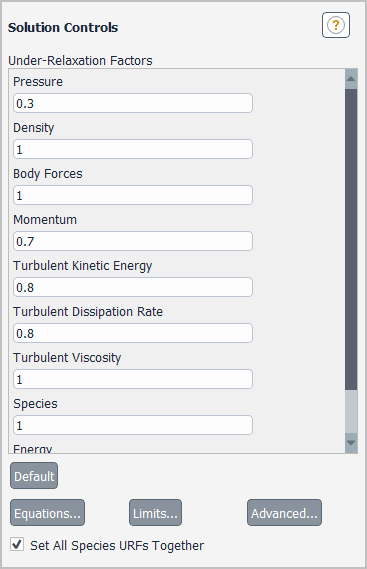
You can set the under-relaxation factor for each equation in the field next to its name under Under-Relaxation Factors.
Important: If you are using the pressure-based solver, all equations will have an associated under-relaxation factor (see Under-Relaxation of Equations in the Theory Guide). If you are using the density-based solver, only those equations that are solved sequentially (see Density-Based Solver in the Theory Guide) will have under-relaxation factors.
If your case involves species transport, you can set the under-relaxation factors for each of the listed species. If you want all your species to use the same under-relaxation factors, simply enable the Set All Species URFs Together option. Notice that you will no longer see your list of individual species, instead a Species field will appear where you will specify the under-relaxation factor.
If you change under-relaxation factors, but you then want to return to Ansys Fluent’s default settings, you can click the button.
Note that with optimal settings, the convergence of the coupled pressure-velocity algorithm will be limited by the segregated solution of other scalar equations, for example, turbulence. For optimum solver performance, you will need to increase the relaxation factors for these equations to a value greater than the default values.
You can use the non-iterative solver (also referred to as "NITA"—see Time-Advancement Algorithm in the Theory Guide) for transient problems in order to increase the speed and efficiency of the calculations. You can also obtain a steady solution using the non-iterative multiphase solver for multiphase flows with quasi-steady conditions.
To control the change of computed variables at each iteration, you can specify explicit relaxation in the Non-Iterative Solver Relaxation Factors list in the Solution Controls Task Page. Additional information on relaxation factors can be found in Setting Under-Relaxation Factors.
Other solution controls are accessible via the Expert tab, in the Advanced Solution Controls dialog box (see Figure 36.6: The Advanced Solution Controls Dialog Box for the Pressure-Based Segregated Non-Iterative Solver). The criteria for convergence include the Correction Tolerance (defined by the overall accuracy), Residual Tolerance (controlling the solution of the linear equations), and Max. Corrections (controlling the maximum number of sub-iterations for each individual equation). The default control settings are optimally designed in order to get a second-order accurate solution.
To use Ansys Fluent’s non-iterative transient solver in order to boost the efficiency of transient simulations:
Go to the Solution Methods task page.
 Solution →
  Methods
Make sure that Coupled is not selected from the Pressure-Velocity Coupling drop-down list.
Enable Non-Iterative Time Advancement.
Under Pressure-Velocity Coupling, select a scheme from the drop-down list:
For single phase or VOF/Mixture multiphase flows: You can select either the Fractional Step or PISO scheme. For the PISO scheme, you can set the value for the Neighbor Correction; the value for skewness correction is determined automatically with the goal of convergence of the pressure equation (to print these "pressure correction equations" in the console during the solution, you can increase the multigrid verbosity using the
solve/set/multi-grid-amgtext command).For Eulerian multiphase flows: Select the Phase Coupled SIMPLE scheme. This is the only pressure scheme for Eulerian multiphase simulations that allows the NITA option.
When using the Large Eddy Simulation (LES) turbulence model, you can enable the Accelerated Time Marching option in order to speed up the simulation. This option is intended for unreacting flow simulations that use a constant-density fluid. It enables a modified NITA scheme and changes the following to a more aggressive setting:
The maximum number of sub-iterations for the NITA solver equations (specified in the Expert tab of the Advanced Solution Controls dialog box) are revised: the Max. Corrections is set to
0for Pressure and1for all other equations.The pressure-velocity coupling scheme (specified in the Solution Methods task page) is changed to the Fractional Step method.
The multigrid solver settings (specified in the Multigrid tab of the Advanced Solution Controls dialog box) are revised: for the Pressure equation, the Cycle Type is changed to F-Cycle and the Termination criterion is set to
0.01.
Note: The following limitations / recommendations apply:
The accelerated time marching option is not available with the Eulerian multiphase model.
It is not recommended for compressible or variable-density fluids.
When using this option, it is recommended that you use the Bounded Central Differencing scheme for the Momentum equation rather than the Central Differencing scheme.
You can modify the under-relaxation factors in the Solution Controls Task Page (Figure 36.5: The Solution Controls Task Page for the Pressure-Based Solver).
![]() Solution →
Solution → ![]() Controls
Controls
The relaxation factors define the explicit relaxation (see Under-Relaxation of Variables in the Theory Guide) of variables between sub-iterations. The relaxation factors can be used to prevent the solution from diverging.
If the solution is unstable:
For single phase flows: You should first try to stabilize the solution by lowering the relaxation factors for pressure to 0.7–0.8, and by reducing the time step size.
For multiphase flows: Consider lowering the explicit pressure relaxation factor up to 0.5. This may help when meshes are poor, because a poor mesh will significantly affect the pressure gradient, which in turn may generate large source terms in the governing equations resulting in poor convergence. You can set the under-relaxation factors for the other flow variables to higher values (0.8-1.0). For compressible multiphase flow, you can use explicit relaxation of density in the range 0.5-0.8. For multiphase cases with mass transfer, you can use explicit relaxation of vaporization mass in the range 0.5-0.8.
You can modify the non-iterative solution controls in the Advanced Solution Controls Dialog Box (Figure 36.6: The Advanced Solution Controls Dialog Box for the Pressure-Based Segregated Non-Iterative Solver).
![]() Solution →
Solution → ![]() Controls →
Advanced...
Controls →
Advanced...
Figure 36.6: The Advanced Solution Controls Dialog Box for the Pressure-Based Segregated Non-Iterative Solver
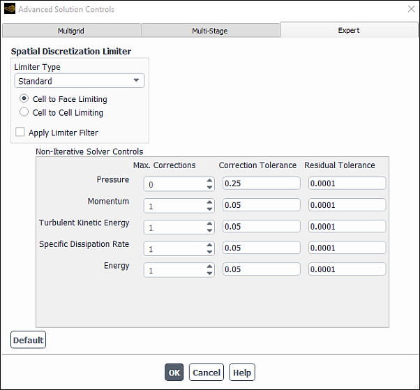
Under Non-Iterative Solver Controls, there are several parameters that control the sub-iterations for the individual equations.
The sub-iterations for an equation stop when the total number of sub-iterations exceeds the value specified for Max. Corrections, regardless of whether or not the convergence criteria (described below) are met.
The sub-iterations for an equation end when the ratio of the residuals at the current sub-iteration and the first sub-iteration is less than the value specified in the Correction Tolerance field. You can monitor the details of the sub-iteration convergence by looking at the AMG solver performance (that is, setting the Verbosity field in the Multigrid tab in the Advanced Solution Controls dialog box to 1). Be sure to pay attention to the residuals for the current sub-iteration (that is, the residual for the 0-th AMG cycle at the current sub-iteration) and the initial residual of the time step (that is, the residual for the 0-th AMG cycle of the first sub-iteration). The ratio of these two residuals is what is controlled by the Correction Tolerance field. These two residuals are also the residuals plotted when using the Residual Monitor panel and reported in the Ansys Fluent console at the end of a time step. Note that the residuals reported at the end of a time step can be scaled or unscaled, depending on the settings in the Residual Monitor dialog box. The residuals reported when monitoring the AMG solver performance are always unscaled.
For each interim sub-iteration, the AMG cycles continue until the usual AMG termination criteria (0.1 by default, and set in the Multigrid tab) are met. However, for the last sub-iteration (that is, either when the maximum number of sub-iterations are reached or when the correction tolerance is satisfied), the AMG cycles continue until the ratio of the residual at the current cycle to the initial residual (the residual for the 0-th AMG cycle of the first sub-iteration of the time step) drops below the value specified for Residual Tolerance. You may want to adjust the Residual Tolerance, depending on the size of the time step selected. The default Residual Tolerance should be well suited for moderate-sized time steps (that is, for cell CFL numbers of 1 to 10). Note that you can display the cell CFL numbers for unsteady problems by selecting Cell Courant Number in the Velocity... category of all postprocessing dialog boxes. For very small time steps (cell CFL <<1), the diagonal dominance of the system is very high and the convergence should be driven further by reducing the Residual Tolerance value. For larger time steps (cell CFL >>1), it may be possible that the residual tolerance cannot be reached due to round-off errors, and unless the Residual Tolerance value is increased, AMG cycles can be wasted. Again, this can be monitored by monitoring the AMG solver performance.
For NITA cases that involve VOF or Mixture multiphase model, the Hybrid NITA option may help you improve solution stability and robustness, but at the cost of speed. Depending on your case, the hybrid NITA settings may optimize NITA expert controls, AMG settings, explicit relaxation factors, pressure interpolation scheme, neighbor corrections for PISO, and outer iterations.
To enable and edit the Hybrid NITA settings:
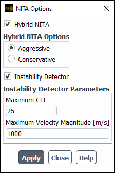
In the Solution Methods task page, enable the Non-Iterative Time Advancement option and click the button next to it.
In the NITA Options dialog box that opens, enable Hybrid NITA.
In the Hybrid NITA Options group box, select from of the following options:
Aggressive : (default) Uses two outer iterations per time-step
Conservative : Uses three outer iterations per time-step
For each option, NITA settings are automatically optimized and, in general, do not require modification for VOF or Mixture multiphase cases.
In case of divergence when using NITA, you can enable Instability Detector.
The hybrid NITA solver performs a fixed number of outer iterations. However, in case of local instabilities during the simulation arising due to meshing events or physical phenomena, large errors may accumulate due to insufficient convergence. The instability detector helps with possible instability problems.
The instability detector traces local instabilities using the following Instability Detector Parameters :
Maximum CFL : Is the maximum of advective Courant number for the instability detection (default = 25)
Maximum Velocity Magnitude : Is the maximum of the velocity magnitude for the instability detection (default - 1000 m/s)
The case when the local Courant number exceeds Maximum CFL, or the local velocity magnitude exceeds Maximum Velocity Magnitude will be considered as an unstable event. The solver will increase the number of outer iterations for that time step and will make some internal adjustments for stability.
With the Hybrid NITA option enabled, you can use additional advanced hybrid NITA controls to improve stability. They can be accessed via the following text command:
solve/set/multiphase-numerics/advanced-stability-controls/hybrid-nita/
The following controls are available:
CFL Type
By default, the instability detector operates on the global advective CFL number calculated in the whole domain. You can change to the interfacial advective CFL definition using the following command:
solve/set/multiphase-numerics/advanced-stability-controls/hybrid-nita/instability-detector/set-cfl-typeAdvective CFL type [0: Global, 1: Interfacial] (0 1) [0]1Initial outer iterations
In most transient applications, the initial conditions do not satisfy continuity. Therefore, being conservative at the start of simulation can help provide better solution stability. By default, Ansys Fluent uses 5 outer iterations for initial 5 time-steps. If necessary, you can change these settings using the following text command:
solve/set/multiphase-numerics/advanced-stability-controls/hybrid-nita/initial-outer-iterations
Number of initial time-steps [5]
Number of initial outer iterations [5]
Note: Initial outer iterations will overwrite outer-iterations for initial time-steps as specified, if initial outer iterations are larger than outer iterations.
Outer iterations for an unstable event
To increase the number of outer iterations for an unstable event, use the following text command:
solve/set/multiphase-numerics/advanced-stability-controls/hybrid-nita/instability-detector/unstable
-event-outer-iterations
By default, the NITA solver uses 5 outer iterations.
Outer iterations
By default, the hybrid NITA scheme provides either 2 or 3 outer iterations for the
1 - aggressiveand2 - conservativeoptions. You can increase the number of outer iterations for certain complex applications using the following text command:solve/set/multiphase-numerics/advanced-stability-controls/hybrid-nita/outer-iterations Number of outer iterations [2]
Note, however, that this will increase the solution run time.
Note: Currently, the residual reports display two residuals for each outer iteration.
Solution Strategies
It is generally not recommended to change the explicit relaxation factors and expert controls for NITA because improper convergence may lead to accumulation of errors and unphysical results. In case of divergence when using NITA, the following strategies may help:
Enable the instability detector and optimize inputs for the Maximum CFL and Maximum Velocity Magnitude.
Use the conservative option for Hybrid NITA.
Reduce the pressure relaxation factor to up to 0.5.
Reduce the time step size.
For cases that involve strong inter-equation coupling (as in mass transfer, compressible flow, and highly viscous flow), using the Conservative option for Hybrid NITA is recommended.
For the Mixture multiphase model, if you are solving for slip velocities, you can specify the explicit relaxation factor for Slip Velocity in the Solution Controls task page.
To obtain diagnostics on convergence of sub-iterations for individual equations, use the following text command:
solve/set/nita-expert-controls/set-verbosityverbosity [0]1The output information may help you to judge whether the specified number of sub-iterations is sufficient to reach the correction tolerance and also to diagnose the source of the solution divergence.
For NITA cases with PISO selected as a Pressure-Velocity Coupling scheme, you can enable coupling of the neighbor and skewness corrections with the following TUI command:
solve/set/nita-expert-controls/skewness-neighbor-couplingenable skewness neighbor coupling for nita [no]yesFor more information about this option, see Skewness - Neighbor Coupling in the Fluent Theory Guide.
The following is a list of models that are compatible with the non-iterative time advancement solver:
Inviscid flow (excluding ideal gas)
Laminar flow
All models of turbulence (including LES and DES)
S2S radiation model
Heat transfer
Non-reacting species transport
General compressible flows (most subsonic and some transonic applications)
VOF multiphase model (most applications)
Mixture multiphase model
Eulerian multiphase model
Phase change (solidification and melting)
Porous media model (isotropic resistance)
Multiphase model with Multi-Fluid VOF
Multiphase RSM turbulence model
The following is a list of models that are compatible with the non-iterative solver, but may result in some instabilities and inaccuracies for certain flow conditions:
RSM turbulence model
MDM
Non-Newtonian fluids
General compressible flows (aerospace supersonic applications)
Reacting species and any type of combustion including PDF
The following is a list of models that are not compatible with the non-iterative solver:
Radiation models (except S2S)
DPM, spark, and crevice models
UDS transport
Porous jump
Porous media model (anisotropic resistance)
RSM turbulence model
Floating operating pressure
Important:
The PRESTO! pressure interpolation scheme, when used with the non-iterative time-advancement solver, is less stable than in the case of the iterative time-advancement solver. As a consequence, a smaller time step size may be required.
As mentioned above, the default control settings are optimally designed to obtain a second-order solution. In order to save CPU time, in cases where transient accuracy is not a main concern (that is, first-order integration in time and space), or when NITA is used to converge toward a steady-state solution, you may want to set the Max. Corrections value to
1in the Advanced Solution Controls dialog box (Expert tab) for all transport equations except pressure.
For transient simulations that use the pressure-based solver, the order in which the model equations are solved can affect the speed of convergence. You can specify the equation order using the following text command:
solve → set → equation-ordering
Note that the standard method is enabled by default and corresponds to the ordering shown in Figure 23.7: Overview of the Iterative Time Advancement Solution Method
For the Segregate Solver and Figure 23.8: Overview of the Non-Iterative Time Advancement Solution Method in the Theory Guide ; alternatively, you can select the
optimized-for-volumetric-expansion method, which is recommended for flows in which the density is strongly
dependent on thermal effects, chemical composition, and so on (such as combustion simulations). This text command is not available
when a multiphase model is enabled.
For simulations that use the pressure-based solver, a correction form of the discretized momentum equation (as described in Correction Form Discretization of the Momentum Equations in the Theory Guide) is used by default. The correction form includes the following advantages:
Avoids floating point error accumulation while collecting source terms, such that equations with large source terms are numerically more robust.
Allows for more simulations to be performed using single precision.
Increases the robustness of the pressure-based coupled solver.
Increases the speed of the pressure-based coupled solver.
Becomes more aligned with the density-based coupled solver.
You can disable the use of the correction form by using the following text command:
solve → set → advanced →
correction-form
Note: In a future release it will not be possible to disable the correction form, and the previous text command will be removed.