You can create multiple Curvilinear Coordinate Systems (CCS) for use in setting up Ansys Fluent cases.
The CCS feature allows you to create local coordinate systems that follow the geometry of the model. For example, you can create a CCS where one of the directions follow the curved shaped of a motor winding. This is especially useful for defining anisotropic thermal conductivity, as described in Anisotropic Thermal Conductivity with Curvilinear Coordinate System (CCS).
Define a CCS using the following steps:
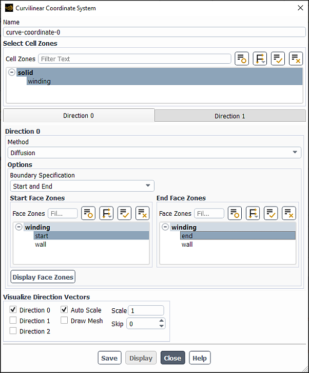
Open the Curvilinear Coordinate System dialog box.
 Setup →
  Curvilinear
Coordinate System
Curvilinear
Coordinate System New...
Under Name, enter a name for the CCS.
Under Select Cell Zones, select the cell zones for which you want to define the CCS.
Define directions for the CCS. Direction 0 and Direction 1 must be specified. Direction 2 is computed automatically using the cross product of Direction 0 and 1.
For Direction 0 and Direction 1, you must specify the direction using the geometry in the chosen cell zone.
Under Method, choose one of the following options:
Diffusion- The direction of the vector field is specified with Start and End face zones. If the geometry is a closed loop, you can use the Jump boundary by specifying a coupled wall as a cross section though the loop, which is then split into start and end faces.Base Vector- You have the option of specifying user defined vectors if you know one of the directions is aligned with the global coordinate system over the entire geometry.Vector Projection(available only for Direction 1) - Requires the specification of the X, Y, and Z components of an Alignment Vector. The direction of the vector field is defined by the projection of the alignment vector onto the principal vector field (Direction 0).Important: The accuracy of the Vector Projection method is dependent on the specified Alignment Vector and principal vector (Direction 0), therefore it is highly recommended that you visualize and verify the computed vectors when using the Vector Projection method. For example on the importance of visualizing the vector fields, see Curvilinear Coordinate System Example.
Under , there are various options to affect how the CCS is displayed in the graphics window.
Direction 0 - Selects Direction 0 to display in the graphics viewer.
Direction 1 - Selects Direction 1 to display in the graphics viewer.
Direction 2 - Selects Direction 2 to display in the graphics viewer.
Auto Scale - Scales the vectors to an appropriate size.
Draw Mesh - Opens the Mesh Display dialog box.
Scale - Specifies the size of the vectors for display.
Skip - Thins the number of vectors displayed to improve visibility.
Click to visualize the direction vectors.
Note: Direction vectors are not displayed on all interior boundaries.
Click to save the coordinate system.
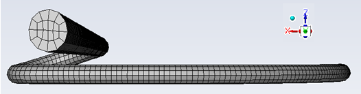
Consider creating a curvilinear coordinate system that follows this coil geometry:
For Direction 0, the
Diffusionmethod can be used with the circular end faces being used as the Start Face Zone and End Face Zone. The result for Direction 0 is a vector field that follows the lengthwise curvature of the coil.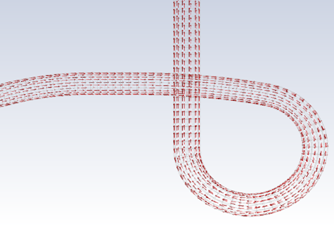
For Direction 1, the
Diffusionmethod cannot be used because there is only a cylindrical face (no start or end face exists). If theBase Vectormethod was used with the direction vector in +Z direction (0,0,1), Direction 1 would still not be aligned with curvature of coil.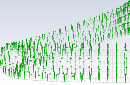
For Direction 1, the
Vector Projectionmethod should be used to align the secondary direction with the curvature of the coil. Specifying the Alignment Vector in the +Z direction (0,0,1) ensures that the vector field for Direction 1 is normal to Direction 0.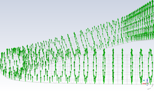
The following limitations exist for Curvilinear Coordinate Systems:
Periodic Boundary face zones are not available in the Face Zone lists for selection of Start, End Jump condition faces.
Jump boundaries are valid for closed-loop geometries only.
An open ended geometry with jump boundary will lead to incorrect results. See below for an example of an open-ended geometry. Left and right sides are open, and jump is provided on a coupled wall in between two cell zones C1 and C2.

Closed loops cannot have more than one jump boundary.
In the example below, there are four cell zones CZ1, CZ2, CZ3 and CZ4, and 4 coupled walls CW1, CW2, CW3 and CW4. You can only specify one coupled wall inside the closed loop geometry as the jump boundary (CW4 in this case).
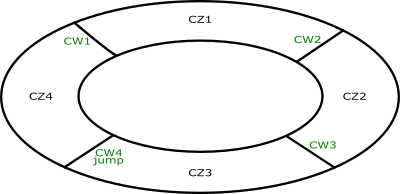
Using the same example, you cannot have all coupled walls with same thread ID. In such a scenario, specifying a jump boundary on one of the coupled walls would result in all four coupled walls having a jump boundary, invalidating the condition of only one jump per closed loop.
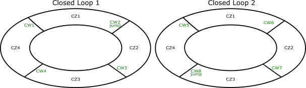
Considerations for multiple closed loops
Multiple closed loops with the same thread ID for coupled walls can work only if one coupled wall is selected as the jump boundary (CW2 in example below). Only one of CW1, CW2, CW3 or CW4 can be selected in this case. Otherwise, there would be more than one jump boundary in each closed loop.
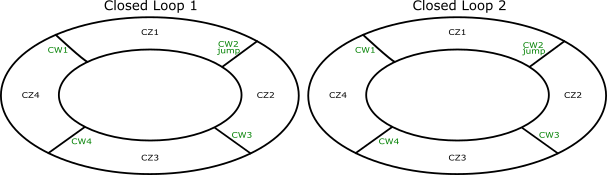
If different closed loop geometries have different coupled wall thread IDs, then you can select one of the coupled walls in each loop as the jump boundary (CW2 and CW8 in example below).