


The forced vibration analysis in turbomachinery (a.k.a. Forced Response Analysis) is essential for predictions of blade structural failures. An important ingredient in this analysis is the prediction of the blade aerodynamic damping value from blade flutter analysis. The aerodynamic damping value is directly impacted by the severity and characteristic of the vibration and the nature of the blade response.
Blade flutter usually occurs at the natural frequency of the blade-disc assembly. This natural frequency can be determined, along with blade displacements (mode-shapes), using Modal analysis in Ansys Mechanical (or other third party FEM software) prior to performing a flow analysis on the blade. In general, a rotor-disc assembly can have many vibration modes. However, only a limited number of these modes contribute to flutter and only these modes are considered in a blade flutter simulation setup.
Ansys Fluent offers two methods for the calculation of the aerodynamic damping value: the Travelling Wave Method and the Influence Coefficient Method.
A typical process to set up a blade flutter simulation follows:
Set-up a steady-state case and run it to get a solution that can be used later for initialization purposes.
Read the mode-shape profile file.
For details, see Reading the Mode Shapes.
Configure Run Calculation settings.
 Solution → Run
Calculation →
Solution → Run
Calculation →
For details, see Configuring Run Calculation Settings.
Set up dynamic mesh zones that impose blade flutter and other movement specifications on the boundaries.
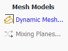
Enable Dynamic Mesh for the domain as described in Turning on Dynamic Mesh.
On the Periodic Displacement tab, define periodic displacement settings as described in Defining the Periodic Displacement of the Blades.
Assign proper motion specifications to every boundary as described in Creating and Applying Dynamic Mesh Zones.
For details, see Using Dynamic Mesh Zones in a Blade Flutter Simulation.
Important: It may be necessary to initialize the flow field immediately after specifying the dynamic mesh zones and before specifying any Report Definitions, otherwise you maybe receive an error message. This is due to data required by the Report Definitions only getting interpolated to the blades when the flow is initialized.
Set up solution monitors for aerodynamic damping.
Solution
→ Reports → Definitions
→ New → Aeromechanics
ReportThere are separate reports available for the Travelling Wave Method and the Influence Coefficient Method.
For details, see Common Postprocessing for a Blade Flutter Case.
The blade displacements (mode shapes) for a blade flutter case are encoded in a mode shape profile file, which can be obtained by performing a modal analysis in Ansys Mechanical or third-party FEM software.
For more information on how to export mode shape profiles from Ansys Mechanical, see the following APDL commands:
A mode shape profile file from Ansys Mechanical has a .csv file extension and can be read as you would a regular boundary profile:
For details on reading profiles, see Reading Profile Files.
The format expected by Fluent is a file that lists:
[Name] - The name of the mode shape profile.
[Parameters] - Parameters for various data that can be used during run setup. For example, the frequency of the mode shape is reported by Ansys Mechanical in the profile, which can then be used in the blade displacement definition. For details, see Defining the Periodic Displacement of the Blades.
[Data] - The normalized or non-normalized displacement values with real only (or with real and imaginary) components.
[Faces] - Contains face connectivity information which allows you to preview the profile in the graphics window as a surface, which can be useful to ensure the profile is oriented correctly. To do this, click Preview on Figure 7.96: The Profiles Dialog Box. For details on reorienting a profile, see Reorienting Profiles.
Passage number (or sector tag) information is also required. This field is added as an additional column in the [Data] section of the profile. It is automatically generated when the profile is replicated from its original single passage modal shape calculation. For details on replicating a profile, see Replicating Profiles.
The passage number is independent of machine rotation and starts with a value of one for the original passage and increases around the wheel in a direction established using the right hand rule and the global coordinate frame, as shown in figure Figure 14.9: Passage Numbering from Profile Expansion.
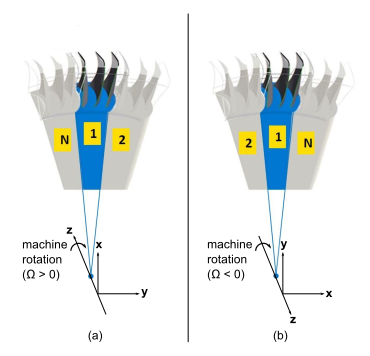
The machine rotation can be specified either as cell zone Frame Motion or Mesh Motion as described in Defining Zone Motion. In the case of Mesh Motion, extra care must be taken to ensure the profile is aligned with the zone mesh throughout the simulation. Therefore, a local reference frame must be defined and set with the same rotation speed and direction as the zone. For details on specifying a local reference frame, see Creating and Using Reference Frames.
Important: When a combination of cell zone Mesh Motion and Periodic Displacement with profiles is used, Fluent checks if a local reference frame is set and tracking the zone (that is, same rotation and direction as the cell zone). If this requirement is not met, Fluent prompts you to create a local reference frame and link it to the profile that is being used in the Periodic Displacement.
Here is an abbreviated example of a valid mode shape profile file (with "..." representing omitted similar lines):
[Name]
modeshape1

[Parameters]
Ncompt = 3
Nnodes = 9080
Mass = 3.64422308E-002 [kg]
Frequency = 1075.7960 [Hz]
Maximum Displacement = 19.161390 [m]

[Spatial Fields]
Initial X [m], Initial Y [m], Initial Z [m]

[Data]
Initial X [m], Initial Y [m], Initial Z [m], norm meshdisptot x [ ], norm meshdisptot y [ ], norm meshdisptot z [ ]
 0.24326721     ,  2.31312828E-002,  3.40935170E-002,  6.64623727E-002, -0.29486747     ,  0.26849515
 0.24326396     ,  2.31793349E-002,  3.40879478E-002,  6.70239889E-002, -0.29487824     ,  0.26807998
 0.25071740     , -2.49000213E-002,  6.40013147E-003, -0.11782411     , -0.61531118     ,  0.77716603
 0.25072379     , -2.48944600E-002,  6.37840505E-003, -0.11739263     , -0.61562871     ,  0.77721180
 0.25073487     , -2.48733125E-002,  6.34503139E-003, -0.11655654     , -0.61613393     ,  0.77716960
...
[Faces]
         127,          128,          377,          378
         706,          455,          456,          705
         128,          375,          376,          377
         705,          456,          457,          458
         127,          410,          129,          128
         706,          705,          704,          423
         415,          410,          127,          126
         418,          707,          706,          423
...For the Time Advancement settings in the Run Calculation task page:
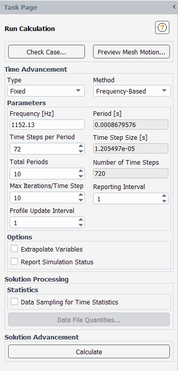
For details on this task page, see Run Calculation Task Page.
To apply blade flutter, you can set up dynamic mesh zones and apply them to the boundaries. The dynamic mesh zones that are applied to the wall surfaces are driven according to periodic displacement settings that involve the Aerodynamic Damping option.
Blade flutter is applied to the blades using Dynamic Mesh. You must enable Dynamic Mesh before you can define the Periodic Displacement for the blades.
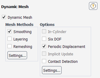
With Dynamic Mesh turned on, you are ready to define the Periodic Displacement for the blades. When Periodic Displacement is set, Fluent automatically turns on the Mesh Smoothing method. The recommended Mesh Smoothing Methods are, in order of preference:
Linear Elastic Method (with a Poisson’s ratio of 0.45)
Diffusion Method (with diffusion parameter of 1.5)
On the Dynamic Mesh task page, under Options, select Periodic Displacement, and click Settings.
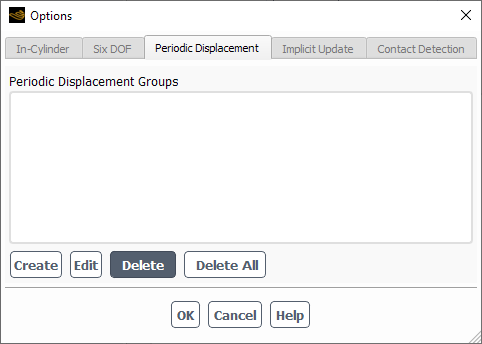
In the Options dialog box, on the Periodic Displacement tab:
To create a new Periodic Displacement Group, click Create. You can create as many groups as needed. This allows you to quickly run different mode shapes by having different displacements activated under each group. Existing Periodic Displacement Groups can be modified by clicking Edit or deleted with Delete or Delete All.
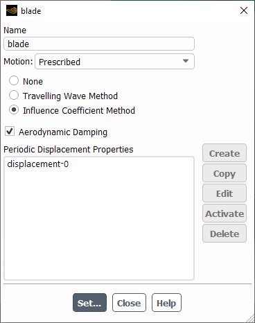
Clicking Create opens the Periodic Displacement Group dialog where you can assign a name to group and specify some setting common to that group. Clicking Set... saves the settings for the group.
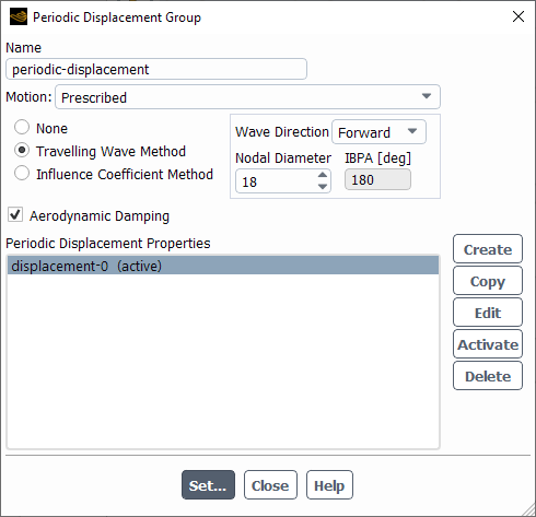
If you are editing an existing group, a dialog box appears for the selected group where you can specify some settings related to the motion of the blade.
The Motion can currently only be set as
Prescribedwith no wave (None) or one of the following options:Travelling Wave Method. For details, see Traveling Wave Method (TWM).
Influence Coefficient Method. For details, see Influence Coefficient Method (ICM).
This will enable monitoring of the damping factor in postprocessing. Aerodynamic Damping is automatically enabled for new groups. See TWM Method Post-processing for more details.
Create one or more periodic displacements under Periodic Displacement Properties. All currently defined periodic displacements will appear under each Periodic Displacement Group, however you must activate one periodic displacement for each group. After selecting the displacement you want to make active for a particular group, click Activate. The
(active)suffix will appear next to the currently active displacement.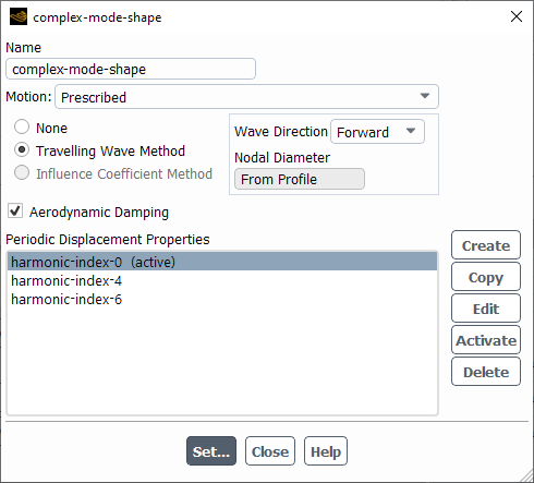
You can also copy an existing displacement by selecting the original displacement you want and clicking Copy. The copied displacement will have the same settings as the original, but with the default displacement name (which can be changed at any time). To specify a new displacement, click Create and a dialog box will appear to specify the displacement.
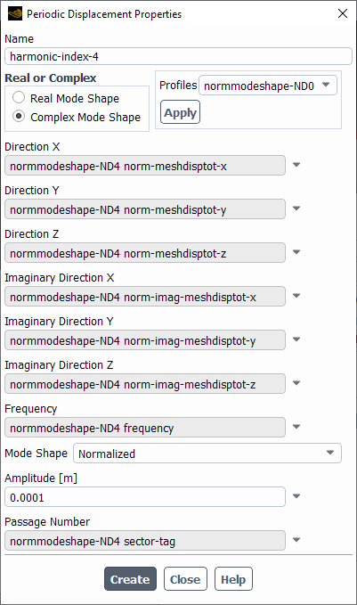
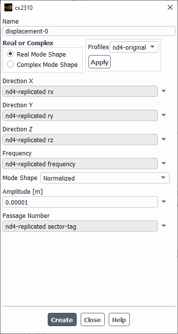
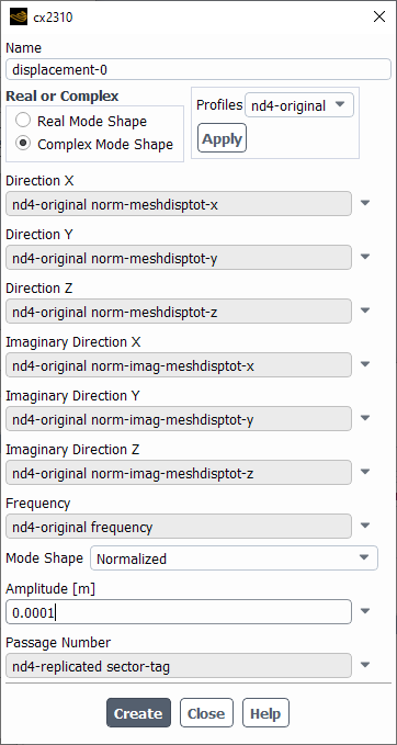
In the Profiles group box, all loaded profiles that contain the mesh displacement field variables (variables containing the meshdisp, meshdisptot keyword) can be selected. After selecting a profile from the drop-down list and clicking Apply, the dialog box will be filled based on the profile. Parameter values present in the profile such as mode shape frequency, and amplitude, if present, are also automatically applied to their respective fields. Otherwise, you can follow the steps below to specify a periodic displacement manually.
Specify the mode shape as Real or Complex.
Specify the displacement components (real and imaginary, if applicable) by setting Direction X, Direction Y, Direction Z (and Imaginary Direction X, Y, and Z, if applicable) using the mesh displacement variables from the
.csvfile (as described in Reading the Mode Shapes), via UDF, or using an expression. For details on specifying the displacement components using a UDF, seeDEFINE_PERDISP_MOTIONin the Fluent Customization Manual. An example for specifying the displacement components with an expression is shown below: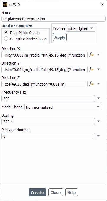
The expression for Direction X is broken down in the following table:
Function: Equivalent Expression: 
-inity*0.001[m]/radial*sin(49.15[deg])*function
sqrt(initx^2+inity^2)
6.3*10^-2*radial*1[m^-1]-5.94*10^-3
x-XTotalMeshDisplacement
y-YTotalMeshDisplacementSet Frequency to the mode shape frequency.
This frequency is among the data that is deleted from the original profile file (as output by Mechanical) while creating a profile file suitable for loading into Fluent.
Set whether the mode shape is Normalized or Non-normalized.
Set Amplitude (for normalized mode shapes) or Scaling (for non-normalized mode shapes).
For normalized mode shapes, Fluent requires the Amplitude value. The Amplitude multiplies the provided normalized (maximum amplitude of 1.0) dimensionless modal displacement values by the specified amplitude in order to obtain the maximum modal displacement values. The recommended starting value for the Amplitude is 0.05% of the blade chord length.
For non-normalized profiles, Fluent requires the Scaling value. The Scaling parameter scales the displacement vector by the value specified in the Scaling field. The recommended starting Scaling value is 0.5.
It is recommended that you preview the mesh motion with the recommended settings of Amplitude or Scaling factor and Mesh Methods using the desired time step size and at least for the same number steps in one vibration period. The mesh preview feature is located at the bottom of the Dynamic Mesh task page.
Domain → Mesh
Models → →
Set Passage Number to the sector tag variable from the .csv data. For more details, see Reading the Mode Shapes.
This provides an integer that identifies each blade. In the case of the Travelling Wave Method, this is required for the proper specification of the IBPA. In the case of the Influence Coefficient Method, this blade numbering is a requirement of the aerodynamic damping calculation.
An example of a Periodic Displacement specification from a real mode shape is shown below.
An example of a Periodic Displacement specification from a complex mode shape with frequency from the profile parameter is shown below.
With Periodic Displacement defined for the blades, you are ready to specify the motion of the blades and other boundaries. To do this, you need to create and apply dynamic mesh zones.
To create a dynamic mesh zone:
Details for the required dynamic mesh zones:
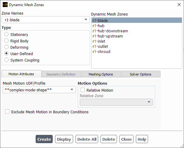
To impose vibration on the blades:
In the Dynamic Mesh Zones dialog box, set Type to User-Defined.
On the Motion Attributes tab, set Mesh Motion UDF/Profile to a Periodic Displacement Group specified early as described in Defining the Periodic Displacement of the Blades.
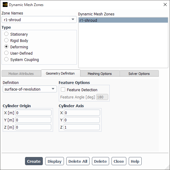
For cases that involve blade tip gaps, it is beneficial to allow the mesh surface across the gap from the blade tip to slide freely along a surface of revolution.
In the Dynamic Mesh Zones dialog box, set Type to Deforming.
On the Geometry Definition tab, set Definition to
surface-of-revolution.This option prevents the mesh elements in the gap from becoming skewed by allowing the mesh nodes on the shroud to "slide" as the mesh follows the motion on the blade tip, while preventing the gap thickness from changing.
Ensure that the Cylinder Axis components (X, Y, Z) indicate the correct direction for the axis. These components are not automatically set according to your simulation.
Note: Currently, tip gap with interfaces are not supported with the Periodic Displacement method. A tip gap without interfaces can be accommodated with the proper specification of the shroud boundary condition.
Hub
Typically, the hub is set as stationary. However, for cases that involve complex mode shapes, the hub surface may have to be added to the list of surfaces that undergo the periodic displacement motion. For such a case, you can set the hub in the same way as was done for the blades:
In the Dynamic Mesh Zones dialog box, set Type to User-Defined.
On the Motion Attributes tab, set Mesh Motion UDF/Profile to a Periodic Displacement Group specified early as described in Defining the Periodic Displacement of the Blades.
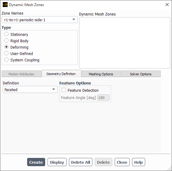
Rotational Periodic Boundaries
Typically, rotational periodic boundaries are set as stationary.
For cases where the rotational periodic boundaries are connected to other surfaces that undergo periodic displacements, it is important to allow the periodic boundaries to move and match the displacement, especially on the shared nodes. This is common in cases involving complex mode shapes. In such cases, the Deforming type with the Faceted definition is recommended.
In the Dynamic Mesh Zones dialog box, set Type to Deforming.
On the Geometry Definition tab, set Definition to
faceted.
If no motion is expected on the rotational periodic boundaries, you may set the Type to Stationary.
For the other boundaries, set Type to Stationary. Note that if boundaries are left unspecified, they will automatically be defined as Stationary.
For details on dynamic meshes, see Modeling Flows Using Sliding and Dynamic Meshes.
To predict the aerodynamic damping, the TWM is employed in modeling the blade flutter analysis. In TWM, the mesh displacement is prescribed on all the blades in the model. The blades are assumed to vibrate with a frequency equivalent to the natural frequency of a blade and with a phase shift between each blade known also as the Inter-blade Phase Angle (IBPA). The IBPA is dependent on the nodal diameter. This vibration pattern behavior results in a traveling wave. A Forward Traveling Wave (FTW) or Backward Traveling Wave (BTW) pattern is the result of lead or lag in the phase of motion from one blade to the next. A FTW is defined as a wave pattern that travels in the direction that the machine rotates, while a BTW is defined as a wave pattern that travels in the direction opposite that the machine rotates.
For blade flutter calculations, it is important to consider the
aerodynamic effects of adjacent blades. For a rotor-disc assembly consisting of
 blades, there is a finite number of disc nodal diameters. At nodal
diameter 0 (
blades, there is a finite number of disc nodal diameters. At nodal
diameter 0 ( ), all the blades vibrate in phase with an Interblade Phase Angle (IBPA) of
0. However, for any other nodal diameter values, each blade will be out of phase with
respect to the adjacent blades by some finite IBPA value. The IBPA can be computed from the
nodal diameter:
), all the blades vibrate in phase with an Interblade Phase Angle (IBPA) of
0. However, for any other nodal diameter values, each blade will be out of phase with
respect to the adjacent blades by some finite IBPA value. The IBPA can be computed from the
nodal diameter:

where  for an even number of blades and
  for an odd number of blades.
The main objective of a blade flutter analysis is to obtain the aerodynamic damping, or work per vibration cycle. Once a transient periodic solution is achieved, you can use the energy balance method to perform the damping calculation. This calculation yields a measure of the system stability at each combination of nodal diameter and blade vibration frequency. The work per vibration cycle can be computed as:
 | (14–2) |


Note: Positive values for work indicate that the vibration is damped (for the combination of nodal diameter and blade vibration frequency being studied), whereas negative values indicate that the vibration is undamped/excited.
Typically, when using the TWM/Energy method to obtain aerodynamic damping, you need two simulations for each nodal diameter possible in the rotor assembly: one for a FTW and one for a BTW.
You can use aerodynamic damping monitors to monitor aerodynamic damping during a run. The monitor value can be calculated using a normalized version of Equation 14–2.
There are three possible setup configurations when modeling Aerodynamic Damping using TWM:
Use a full-wheel model where all the blades in the row are included. With this model topology, the entire range of nodal diameters is modeled using a single problem setup. However, the computational cost is expensive due to the size of the mesh.
Use a periodic sector for specific nodal diameters (periodicity must be achieved). This is a much more economical modeling strategy but the disadvantage is that multiple configurations are needed to cover the entire nodal diameter range. Also, it is not always possible to find a valid periodic sector if there is an odd number of blades in the row.
Use a single passage model and apply a Fourier-based phase-lag boundary condition. With this modeling option, a single setup is used to cover the entire nodal diameter and at the same time, the computational cost is much less than the periodic-sector or full-wheel model due to solving the flow problem on a single passage only. The additional problem setup required for an aerodynamic damping flow problem using a phase-lag boundary condition is described in Phase-lag Method.
In addition to the steps outlined in Common Settings for a Blade Flutter Case, there are some settings that are unique to the TWM method. These settings are outlined below.
Refer to Using Dynamic Mesh Zones in a Blade Flutter Simulation for steps on setup of the Dynamic Mesh and Periodic Displacement.
On the Periodic Displacement Group dialog box, select Travelling Wave Method and Aerodynamic Damping.
With the Traveling Wave Method, additional settings appear for controlling the displacement wave:
Wave Direction:
ForwardorBackwardA forward traveling wave moves in the direction of rotor rotation.
A backward traveling wave moves in the direction opposite of rotor rotation.
Nodal Diameter:
The vibration of the blades with Interblade Phase Angle (IBPA) results in a traveling wave pattern. For complex mode shapes that are generated with cyclic symmetry, the mode shape profile is already phase-shifted so the IBPA is not needed. For real only mode shapes, you must supply information about the IBPA.
For real only mode shapes, the corresponding IBPA is shown to the right of the Nodal Diameter setting. The IBPA is the blade pitch multiplied by the nodal diameter.
The blade pitch is determined by the number of blades, which you can set using the Turbomachinery Description console command. For details, see Turbomachinery Description.
For complex mode shapes, the IBPA is embedded in the mode shape profile. Therefore, the Nodal Diameter setting field is replaced by the non-editable option From Profile. To simulate a different Nodal Diameter, you must obtain another mode shape associated with the desired Nodal Diameter.
Note:Depending on the combination of Nodal Diameter and the total number of blades in the machine, you might have the option to model a periodic sector of the wheel instead of the full wheel.
If splitter blades are involved, then for the purpose of calculating the magnitude of the nodal diameter, the blade pitch should be measured from one main blade to the next.
Create a periodic displacement for the group and complete the remainder of the setup as described in Common Settings for a Blade Flutter Case.
As a prerequisite to the options discussed in this section, you must ensure that the
turbomachine description has been previously specified. This is done automatically if you
set up your case using the turbomachine workflow (as described in Using the Turbomachinery Guided Workflow) or manually with the command
/define/turbo-model/create-turbomachine-description (as
described in Turbomachinery Description).
You have the option to compute the following:
Fourier coefficients of pressure, velocity components, and temperature based on the blade flutter frequency of the simulation.
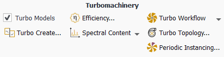
Computing the Fourier coefficients is enabled from the Spectral Content tab in the Turbomachinery ribbon or from the
define/turbo-modelmenu of the console text commands. For details, see General Fourier Coefficient Postprocessing for Turbomachinery Cases.Real and imaginary harmonic pressure loads on surfaces based on the blade flutter frequency of the simulation. This computation is enabled using the following text command:
define/turbo-model/blade-flutter-harmonics/enable-harmonic-exports?By default, the pressure loads will be computed for all boundaries, however, you can also specify which boundaries to use for the calculation.
At the conclusion of the run you can write the harmonic exports
to a .csv file using the following command:
define/turbo-model/blade-flutter-harmonics/write-harmonic-exports?
The results from the aerodynamic damping analysis for the specified nodal diameter and harmonic index (both written in the file in the parameters section) at each surface chosen for harmonic export will be written to a separate file. The file name will be the surface name appended to a root file name that you are prompted for.
Since face connectivity is automatically written into the
.csv file, these files can be read into Fluent (or CFD-Post)
to visualize the export surfaces as well as the real and imaginary first harmonic of
pressure. To do this, after reading the .csv file, click
Preview on Figure 7.96: The Profiles Dialog Box. For details
on reading profiles, see Reading Profile Files.
The harmonic export .csv file is then read into Ansys Mechanical or a
third-party FEM software for a forced response analysis. The file has the following format
(with "..." representing omitted similar lines):
File identification header - Information for documentation and traceability including Fluent version number, date generated, and case file.
[Name] - Name of the profile.
[Parameters] - Various parameters required by Ansys Mechanical.
[Spatial Fields] - Mesh nodal coordinate system.
[Data] - Nodal surface coordinates and real/imaginary pressure harmonics.
[Faces] - Face/node connectivity data for visualization.
## ANSYS Fluent 22.2.0
##
## Generated on: Thu Nov 11 17:47:36 2021
##
## Generated from case: STCF-11_notipgap_TRS_64tspp_s1r.cas.h5
##
[Name]
blade-1

[Parameters]
Ncompt = 1
Nnodes = 3192
Rotation Axis From   = 0.0000000 [m], 0.0000000 [m], 0.0000000 [m]
Rotation Axis To     = 0.0000000 [m], 0.0000000 [m], 1.0000000 [m]
Rotating Speed       = 0.0000 [s^-1 rad]
Frequency            = 209.00000 [Hz]
Nodal Diameter       = -10
Mode Multiplier      = 2.33400000E+02
Travelling Wave Flag = 1

[Spatial Fields]
Initial X, Initial Y, Initial Z

[Data]
Initial X [m], Initial Y [m], Initial Z [m], Passage Number [ ], Real Pressure [kg m^-1 s^-2], Imaginary Pressure [kg m^-1 s^-2], Domain Node Number, Node Number
 1.48709608E-01, -6.25026289E-02, -2.83326356E-02,  1.00000000E+00, -1.58392046E+02,  2.60064686E+01,          1,          0
 1.48834760E-01, -6.22039797E-02, -2.81875705E-02,  1.00000000E+00,  9.35186279E+01,  4.60809849E+01,          2,          1
 1.48281814E-01, -6.20267769E-02, -2.81889840E-02,  1.00000000E+00,  6.91992309E+01,  5.80998775E+01,          3,          2
 1.48157155E-01, -6.23239746E-02, -2.83328554E-02,  1.00000000E+00, -1.87231559E+02,  5.86862670E+01,          4,          3
 1.51736136E-01, -6.24118879E-02, -2.75272228E-02,  1.00000000E+00,  3.36947961E+02, -4.61095015E+01,          5,          4
...
[Faces]
      2925,      2926,      2924,      2922
      2923,      2925,      2922,      2919
      2920,      2923,      2919,      2915
      2916,      2920,      2915,      2910
      2911,      2916,      2910,      2904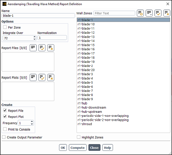
...There is a report definition is available when using the TWM method to monitor the aerodyanmic damping value: Aerodamping (Travelling Wave Method) report definition. As a pre-requisite, you must have Travelling Wave Method) and Aerodynamic Damping selected as described in Defining the Periodic Displacement of the Blades.
Start a new Aerodamping (Travelling Wave Method) report definition from the ribbon:
Solution
→ Reports → Definitions
→ New → Aeromechanics
Report → Aerodamping (Travelling Wave
Method)...
The Aerodamping (Travelling Wave Method) dialog box appears.
If you are modeling multiple (main) blades, select Per Zone so that the damping value is calculated for each dynamic mesh zone (which encompasses one main blade and possibly accompanying splitter blades).
Set Integrate Over to the number of time steps over which to integrate when calculating the damping value; a suggested value is the number of time steps per period.
The number of time steps per period is shown in the Run Calculation task page.
You can also display contours of the TWM aeromechanics related variables (under
Contours of type Aeromechanics).
The Wall Work Density is the work performed on the wall by the fluid per unit of area. It is calculated as:

(14–3)
where
 is the relative mesh displacement and
  is the area unit vector.
The Wall Power Density is the power performed on the wall by the fluid per unit of area. It is calculated as:

(14–4)
where
 is the mesh velocity and
  is the area unit vector.
This method provides a convenient way to calculate the complete range of aerodynamic damping values for all possible nodal diameters supported by the geometry in one Fluent run for a given a real mode shape. In addition, when using this method, you can also calculate and/or visualize the generalized/modal force on any or all blade surfaces involved in the calculation.
The key steps to this calculation are to model a large enough series of consecutively positioned blades and to only oscillate the middle blade while all others are kept stationary. The method relies on the linear superposition principle. The unsteady aerodynamic influences on the middle (reference) blade from all oscillating blades in the blade row are equivalent to the sum of unsteady aerodynamic influence of the middle blade oscillating on itself and on all other stationary blades in the blade row. This permits us to calculate the first harmonic of pressure on the middle(reference) blade in a travelling wave method (TWM) calculation as the sum of the first harmonic of pressure from the oscillating blade itself and its neighboring stationary blades.
In the following equations, n represents the blade
number.
Using superposition principles, we can write the pressure field on a blade at a given inter-blade phase angle as a sum over all the contributions of the n neighboring blades.
 | (14–5) |
From Fourier theory, we can write both the first harmonic of the pressure field and the
periodic displacement vector/mode shape as  ,
,  ,
,  ,
,  . Then we can express the general aerodynamic damping equation
 | (14–6) |
 | (14–7) |
where the generalized/modal forces can be written as:
 | (14–8) |
 | (14–9) |
Note: For sign convention:
The Imaginary part of the pressure force is the opposite sign to the B Fourier coefficient that is accumulated.
Since ICM is for real modes, the B Fourier coefficient for the mesh motion, which can also be expressed as the mode shape, does not need to flip signs (it is just keeping track of the phase and results from using a sin wave for motion that equals 0 at time=0)
In addition to the steps outlined in Common Settings for a Blade Flutter Case, there are some settings that are unique to the ICM method. These settings are outlined below.
Refer to Using Dynamic Mesh Zones in a Blade Flutter Simulation for steps on setup of the Dynamic Mesh and Periodic Displacement.
Specify settings for the periodic displacement group. You must select Influence Coefficient Method and Aerodynamic Damping.
Create a periodic displacement for the group and complete the remainder of the setup as described in Common Settings for a Blade Flutter Case.
The ICM method is only supported for real mode shapes.
The mode shape must be read into Fluent and expanded to cover all blades that will be involved in the calculation.
The blade row modeled must have an odd number of blades. Although only the middle blade will undergo periodic motion at the specified mode shape, this requirement automatically handled in Fluent and all the blades need only to be assigned to the same dynamic mesh displacement group.
There are two reports available when using the ICM method: Aerodamping (Influence Coefficient Method) and Generalized/Modal Force report definitions. As a pre-requisite, you must have Influence Coefficient Method and Aerodynamic Damping selected as described in Defining the Periodic Displacement of the Blades. They are available under:
![]() Solution → Reports
→
→ →
Solution → Reports
→
→ →
Aerodamping (Influence Coefficient Method)
The Aerodamping (Influence Coefficient Method) report definition is used to output the aerodynamic damping values for each nodal diameter. You need to only input the Normalization factor before computing.
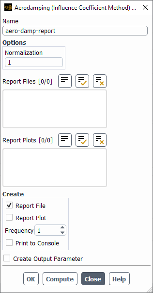
The aerodynamic damping values are reported in the console for each nodal diameter.
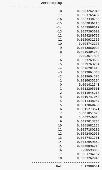
A TUI command is provided to convert the aerodamping file exported by the Aerodamping (Influence Coefficient Method) report definition so that the results can be displayed as Aerodamping value vs Nodal diameter.
define/turbo-model/blade-flutter-harmonics/write-aerodamping-vs-nodal-diameter?
For details on creating plots from a file, see Creating an XY Plot From Multiple Data Sources (Including Files).
Generalized/Modal Force
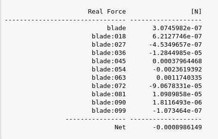
The Generalized/Modal Force report is used to output force on the blade. Under Force Component Type, you can choose to output Real or Imaginary force on the blade. Under Options, you can select Per Zone to conveniently output the force on each blade separately.
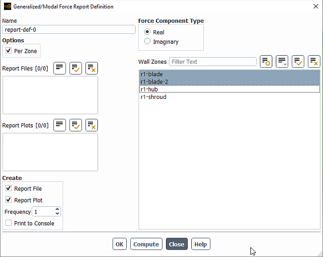
With Per Zone selected, the force will be output for each blade as shown below:
Visualizing Generalized/Modal Force Components
When creating Contours, there are field variables available under the Aeromechanics... section to display the force on the blades.
Real Wall Generalized/Modal Force per Area
Imaginary Wall Generalized/Modal Force per Area
The main goal of a blade flutter simulation is to determine whether the aerodynamic damping value is positive or negative.
The aerodynamic damping is calculated as described in Equation 14–2.
The aerodynamic damping value can be viewed as a report definition monitor or computed in the console using report definitions for the respective method:
For the Travelling Wave Method, see TWM Method Post-processing.
For the Influence Coefficient Method, see ICM Method Post-processing.
Additionally, there are various contour plots that might be of interest:
Display mode shapes of the blade periodic displacement (under Contours of type
Mesh).The interpolated real mode shape profile components (X,Y,Z) are stored in the following variables, respectively:
X Periodic Displacement,Y Periodic DisplacementandZ Periodic Displacement.Likewise, the interpolated imaginary mode shape profile components (X,Y,Z) are stored in the following variables, respectively:
X Imaginary Periodic Displacement,Y Imaginary Periodic Displacement, andZ Imaginary Periodic Displacement.Display the periodic displacement mesh motion variables (under Contours of type
Mesh).The Relative Mesh Displacement is calculated as the difference between the current time step and the previous time step mesh node position. It is stored in the following variables:
X Relative Mesh Displacement,Y Relative Mesh Displacement, andZ Relative Mesh Displacement.The Total Mesh Displacement is calculated as the difference between the current time step and the reference (undeformed) mesh node position. It is stored in the following variables:
X Total Mesh Displacement,Y Total Mesh Displacement, andZ Total Mesh Displacement.