In order to eliminate non-physical pressure wave reflections from boundary zones in a transient simulation for a single-phase, compressible flow with the pressure-based solver, you can designate a layer of the domain adjacent to sets of boundary zones as sponge layers. Within each sponge layer, the density is blended from the value calculated by the solver to a user-specified far-field value. A quadratic blending function gives more weight to the far-field value over a defined ramping length that begins at the interior boundary of the sponge layer and extends toward the boundaries. Such density-based sponge layers are an alternative to the viscosity-based sponge layer (which is only available with the acoustics wave equation model, as described in Using the Acoustics Wave Equation Model) and the boundary acoustic wave models such as NRBCs (as described in Boundary Acoustic Wave Models).
Note: Density-based sponge layers are not supported with a multiphase model.
To use density-based sponge layers, perform the following steps:
Select Pressure-Based for the solver Type in the General task page.
 Setup →
  General
 Select Transient from the Time list in the General task page.
Define a compressible fluid by making an appropriate selection from the drop-down list to the right of Density in the Create/Edit Materials Dialog Box, such as the ideal-gas law, real gas law, or compressible liquid.
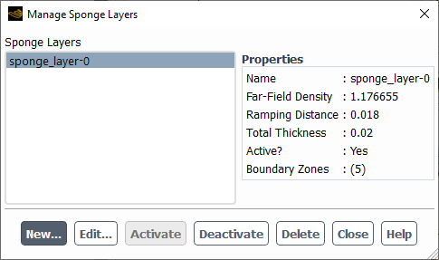
Open the Manage Sponge Layers dialog box.
 Physics → Models
→ Acoustics → Sponge Layers...
Physics → Models
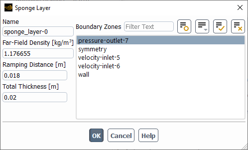
→ Acoustics → Sponge Layers... Click the button to open the Sponge Layer dialog box, where you can define a sponge layer.
Enter a Name for this sponge layer definition.
Enter a value for the Far-Field Density that is used for blending with the solver value. It is recommended that you use the average density at the boundaries throughout the simulation.
Enter a value for the Ramping Distance, a distance over which the density transitions from the solver value to the Far-Field Density. It is recommended that this distance is 80–100% of the Total Thickness.
Enter a value for the Total Thickness of the sponge layer, a distance from the selected boundaries to the interior boundary of the sponge layer. It is recommended that this thickness is at least twice the wavelength of the expected pressure waves.
Make selections from the Boundary Zones list to specify where you want the sponge layer applied.
Click to close the Sponge Layer dialog box.
You can repeat the previous step if you would like additional sponge layer definitions. Whenever you create a new sponge layer, it will automatically be set as active.
Fluent marks sponge layer cells based on the distance from a cell to a sponge layer boundary zone. If there are multiple active sponge layers, then they might overlap. For such cases, Fluent prints a warning message and assigns each cell in the overlapping regions to the sponge layer that has the most distant interior boundary.
After you have created one or more definitions, you can use the Manage Sponge Layers dialog box to take additional actions prior to running the calculation. If you make a selection from the Sponge Layers list, the Properties of the definition are displayed and you can use the buttons at the bottom of the dialog box:
Click to revise the definition of the current selection in the Sponge Layer dialog box.
Click to make the current selection active.
Click to make the current selection inactive.
Click to delete the selected definition.
It can be useful to set up a solution animation of an XY plot of the static pressure near the boundaries, so that you can evaluate if your sponge layers are indeed eliminating the wave reflections. For details, see Animating the Solution and XY Plots of Solution Data.
After initializing the calculation, the following field variables are available for postprocessing (in the Mesh... category):
Sponge Layer Distance
This is the distance from each cell inside a sponge layer to the interior boundary of a sponge layer. It changes linearly from 0 at the interior boundary to the thickness value of the sponge layer at the boundary zone.
Sponge Blending Function
This shows how a blending function changes across a sponge layer, where a value of 0 means the solver density is used and a value of 1 means the far-field value is used.