The steps for setting up a dynamic mesh problem are listed below. (Note that this procedure includes only those steps necessary for the dynamic mesh model itself; you must set up other models, cell zone conditions, boundary conditions, and so on, as usual.)
Enable the appropriate option for modeling transient or steady flow in the General Task Page.
 Setup →
  General
If your problem involves a steady flow, see Steady-State Dynamic Mesh Applications for important considerations.
Set cell zone conditions and boundary conditions as required in the Cell Zone Conditions Task Page and Boundary Conditions Task Page.
Setup → Cell Zone
Conditions
Setup → Boundary
Conditions
See Cell Zone and Boundary Conditions for information about inputting conditions. The correct wall velocity is set up automatically when a dynamic zone is created for a wall zone and the motion attributes are specified, so you will not specify wall motion in the Wall dialog box. If you create a moving dynamic cell zone, then all wall boundaries adjacent to that cell zone will, by default, impose the correct (moving) boundary conditions, and it is not necessary to declare these wall zones as dynamic zones. Note that if a wall boundary mesh is moving because it belongs to an adjacent moving dynamic cell zone, but the physical boundary conditions are such that the wall is actually not moving, then you will have to declare this boundary as a dynamic zone and specify that the mesh motion is not included in the boundary conditions (see Specifying the Motion of Dynamic Zones).
Enable the dynamic mesh model, and specify related parameters in the Dynamic Mesh Task Page.
Setup → Dynamic Mesh →  Dynamic Mesh
See Setting Dynamic Mesh Modeling Parameters for details.
Create the dynamic zones for your model, using the Dynamic Mesh Zones Dialog Box.
Setup → Dynamic Mesh → Create/Edit...
See Specifying the Motion of Dynamic Zones for details.
You can display the motion of the moving zones with prescribed motion to verify the simulation setup.
Setup → Dynamic Mesh → Display Zone Motion...
See Previewing the Dynamic Mesh for details.
If it is a transient simulation, define the events that will occur during the calculation.
Setup → Dynamic Mesh → Events...
See Defining Dynamic Mesh Events for details.
Save the case and data.
 File → Write → Case & Data...
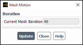
Preview your dynamic mesh setup (when the motion is a prescribed motion). See Steady-State Dynamic Mesh Applications for previewing your steady-state dynamic mesh motion and refer to Previewing the Dynamic Mesh for details.
Setup → Dynamic Mesh → Preview Mesh Motion...
Specify the pressure-velocity coupling scheme. For transient flow calculations, the PISO algorithm is recommended, as it is the most efficient for such cases (see PISO for details).
Use the automatic saving feature to specify the file name and frequency with which case and data files should be saved during the solution process.
Solution → Calculation Activities → Autosave (Every) → Edit...
See Automatic Saving of Case and Data Files for details about the use of this feature. This provides a convenient way for you to save results at successive time steps for later postprocessing.
Important: You must save a case file each time you save a data file because the mesh position is stored in the case file. Since the mesh position changes with each time step, reading data for a given time step will require the case file at that time step so that the mesh will be in the proper position. You should also save your initial case file so that you can easily return to the mesh’s original position to restart the solution if desired.
(optional) If you want to create a graphical animation of the mesh over time during the solution procedure, you can use the Calculation Activities Task Page to set up the graphical displays that you want to use in the animation. See Animating the Solution for details.
(optional) For transient cases, after you have initialized or run the calculation you can use the Moving Mesh Courant Number field variable (in the Velocity... category) to guide your solution. This field variable is a non-dimensional value that indicates the number of cells that might be swept in a single time step due to a mesh motion.
For additional information, see the following sections:
- 13.6.1. Setting Dynamic Mesh Modeling Parameters
- 13.6.2. Dynamic Mesh Update Methods
- 13.6.3. Feature Detection
- 13.6.4. In-Cylinder Settings
- 13.6.5. Six DOF Solver Settings
- 13.6.6. Implicit Update Settings
- 13.6.7. Contact Detection Settings
- 13.6.8. Defining Dynamic Mesh Events
- 13.6.9. Specifying the Motion of Dynamic Zones
- 13.6.10. Previewing the Dynamic Mesh
- 13.6.11. Steady-State Dynamic Mesh Applications
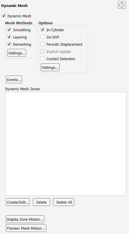
To enable the dynamic mesh model, enable Dynamic Mesh in the Dynamic Mesh Task Page (Figure 13.13: The Dynamic Mesh Task Page).
![]() Setup →
Setup → ![]() Dynamic
Mesh →
Dynamic
Mesh → ![]() Dynamic Mesh
Dynamic Mesh
Then, enable the appropriate options in the Options group box. If you are modeling in-cylinder motion, enable the In-Cylinder option. If you are going to use the six degrees of freedom solver, then enable the Six DOF option. If you want to specify periodic displacement based on a mode shape for blade flutter analysis, select Periodic Displacement. If you want to have the dynamic mesh updated during a time step (as opposed to just at the beginning of a time step), then enable the Implicit Update option. More information about these options and the related settings can be found in In-Cylinder Settings, Six DOF Solver Settings, Defining the Periodic Displacement of the Blades, and Implicit Update Settings, respectively.
Next, you must select the appropriate mesh update methods in the Mesh Methods group box, and set the associated parameters, if relevant. See Dynamic Mesh Update Methods for details.
Three groups of mesh motion methods are available in Ansys Fluent to update the volume mesh in the deforming regions subject to the motion defined at the boundaries:
Note: Smoothing, layering, and/or remeshing are incompatible with mesh adaption.
Details on how to set up the various dynamic mesh update methods are provided in the sections that follow.
When smoothing is used to adjust the mesh of a zone with a moving and/or deforming boundary, the interior nodes of the mesh move, but the number of nodes and their connectivity does not change. In this way, the interior nodes “absorb” the movement of the boundary. To enable smoothing, perform the following steps:
Enable the Smoothing option in the Mesh Methods group box of the Dynamic Mesh Task Page.
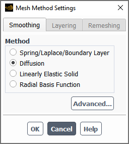
Click the button to open the Mesh Method Settings dialog box.
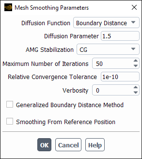
If you want diffusion-based smoothing, select Diffusion from the Method list. Then click the button and define the settings in the Mesh Smoothing Parameters dialog box. For details, see Diffusion-Based Smoothing.
If you want spring-based smoothing, select Spring/Laplace/Boundary Layer from the Method list. Then click the button and define the settings in the Mesh Smoothing Parameters dialog box. For details, see Spring-Based Smoothing.
If you want smoothing using the linearly elastic solid method, select Linearly Elastic Solid from the Method list. Then click the button and define the settings in the Mesh Smoothing Parameters dialog box. For details, see Linearly Elastic Solid Based Smoothing Method.
If you want smoothing that is based on a radial basis function interpolation, select Radial Basis Function from the Method list. Then click the button and define the settings in the Mesh Smoothing Parameters dialog box. For details, see Radial Basis Function Smoothing.
If you selected Diffusion, Linearly Elastic Solid, or Radial Basis Function smoothing and the simulation involves periodic or quasi-periodic motion, you can specify that the smoothing uses a reference position. This option may improve the mesh quality consistency from cycle to cycle—see Smoothing from a Reference Position for details.
If you plan to apply the 2.5D remeshing method (as described in 2.5D Surface Remeshing Method), perform the following steps to set up Laplacian smoothing (as described in Laplacian Smoothing Method).
Select Spring/Laplace/Boundary Layer from the Method list
Click the button and define only the Laplace Node Relaxation and the Maximum Number of Iterations in the Mesh Smoothing Parameters group box (the other settings are not relevant).
If you plan to apply the boundary layer smoothing method (as described in Boundary Layer Smoothing Method), select Spring/Laplace/Boundary Layer from the Method list.
For diffusion-based smoothing, the mesh motion is governed by the diffusion equation
 | (13–2) |
where  is the mesh displacement velocity. The boundary conditions for Equation 13–2 are obtained from the user-prescribed or computed (six
DOF) boundary motion. On deforming boundaries, the boundary conditions are such that the mesh
motion is tangent to the boundary (that is, the normal velocity component vanishes). The
Laplace equation Equation 13–2 then describes how the prescribed
boundary motion diffuses into the interior of the deforming mesh.
is the mesh displacement velocity. The boundary conditions for Equation 13–2 are obtained from the user-prescribed or computed (six
DOF) boundary motion. On deforming boundaries, the boundary conditions are such that the mesh
motion is tangent to the boundary (that is, the normal velocity component vanishes). The
Laplace equation Equation 13–2 then describes how the prescribed
boundary motion diffuses into the interior of the deforming mesh.
The diffusion coefficient  in Equation 13–2 can be used to control how the
boundary motion affects the interior mesh motion. A constant coefficient means that the
boundary motion diffuses uniformly throughout the mesh. With a nonuniform diffusion
coefficient, mesh nodes in regions with high diffusivity tend to move together (that is, with
less relative motion).
in Equation 13–2 can be used to control how the
boundary motion affects the interior mesh motion. A constant coefficient means that the
boundary motion diffuses uniformly throughout the mesh. With a nonuniform diffusion
coefficient, mesh nodes in regions with high diffusivity tend to move together (that is, with
less relative motion).
In Fluent, two different formulations for the diffusion coefficient  are available for selection from the Diffusion Function
drop-down list in the Mesh Smoothing Parameters Dialog Box. The first
formulation allows you to have the diffusion coefficient be a function of the
Boundary Distance, and is of the form
are available for selection from the Diffusion Function
drop-down list in the Mesh Smoothing Parameters Dialog Box. The first
formulation allows you to have the diffusion coefficient be a function of the
Boundary Distance, and is of the form
 | (13–3) |
where  is a normalized boundary distance. The second formulation allows you to have
the diffusion coefficient be a function of the Cell Volume, and is of the
form
is a normalized boundary distance. The second formulation allows you to have
the diffusion coefficient be a function of the Cell Volume, and is of the
form
 | (13–4) |
where  is the normalized cell volume. In both Equation 13–3 and Equation 13–4,
 is a user input parameter. See Diffusivity Based on Boundary Distance and Diffusivity Based on Cell Volume for information about defining the
diffusion coefficient.
is a user input parameter. See Diffusivity Based on Boundary Distance and Diffusivity Based on Cell Volume for information about defining the
diffusion coefficient.
Ansys Fluent uses different numerical methods to solve the vector Equation 13–2, depending on the element types present in the mesh. In
the absence of polyhedral elements or elements with hanging nodes (that is, meshes that have
undergone hanging node adaption and some hexcore or CutCell meshes) the equation is solved
using a finite element discretization and the displacement velocity,  , is obtained directly at each mesh node. If the mesh contains polyhedral
elements or hanging nodes, the equation is discretized using Ansys Fluent’s standard finite
volume method and the cell-centered solution for the displacement velocity,
, is obtained directly at each mesh node. If the mesh contains polyhedral
elements or hanging nodes, the equation is discretized using Ansys Fluent’s standard finite
volume method and the cell-centered solution for the displacement velocity,  , is interpolated onto the nodes using inverse-distance-weighted averaging.
The node positions are then updated according to:
, is interpolated onto the nodes using inverse-distance-weighted averaging.
The node positions are then updated according to:
 | (13–5) |
The finite element discretization is generally superior, as the solution is obtained directly at the nodes and no interpolation step is necessary. The finite volume method can be enforced for meshes of all element types by executing the TUI command:
/define/dynamic-mesh/controls/smoothing-parameters/diffusion-fvm?
      yes
With finite element discretization, you can specify the solution method used by the linear solver for the diffusion-based smoothing calculations. By default, the CG (conjugate gradient) method is selected from the AMG Stabilization drop-down list. This method should be faster in this context than the other available methods, as it takes advantage of the symmetry of the matrix used in the linear systems of equations of finite-element-based mesh smoothing. If divergence is detected with CG, then the generalized minimal residual (GMRES) method will be used for an iteration as a fallback, and you will be informed in the console that a finite-element-based mesh smoothing coupled equation is being stabilized to enhance linear solver robustness. In rare cases, the CG method may result in the generation of negative volume cells; you may be able to avoid this by increasing the Maximum Number of Iterations from the default of 50 to a value in the range of 200–500.
If the CG method continues to generate negative volume cells with a higher number of iterations or if you repeatedly see console messages that say the GMRES fallback is being used, it is recommended that you select GMRES from the AMG Stabilization drop-down list. Note that the GMRES method is more robust than the CG method, especially for high-aspect-ratio meshes; but it is also more demanding in terms of memory usage and solver time.
Note that this drop-down list also allows you to select the BCGSTAB (bi-conjugate gradient stabilized) method; like the CG method, BCGSTAB falls back to the GMRES method for an iteration when divergence is detected.
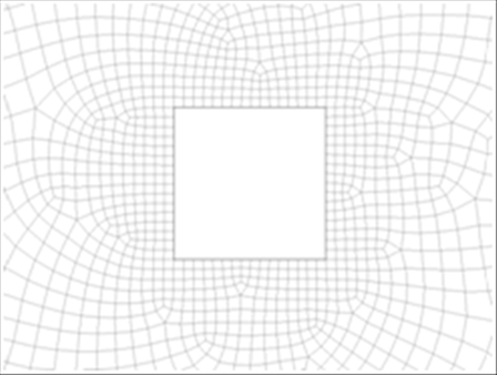
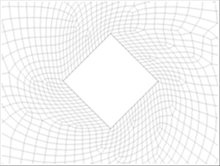
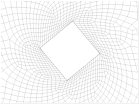
Computationally, solving a PDE for mesh smoothing is generally more costly than spring-based smoothing. But it tends to produce better quality meshes than spring-based smoothing and often allows larger boundary deformations before breaking down. Figure 13.16: The Initial Mesh and Figure 13.17: Valid Mesh After 45 Degree Rotation Using Diffusion-Based Smoothing show a mesh before and after rotating the boundary by 45 degrees, using diffusion-based smoothing. With spring-based smoothing, the same mesh shows degenerated cells after a rotation of 40 degrees (Figure 13.18: Degenerated Mesh After 40 Degree Rotation Using Spring-Based Smoothing). (Note that radial basis function smoothing handles rotation better than both diffusion- and spring-based smoothing.)
It should be noted that with diffusion-based smoothing the interior mesh motion is
governed by the solution to Equation 13–2 and the prescribed
boundary motion, and not by mesh irregularities. Poor quality elements or mesh defects are not
smoothed out by this method, but rather move together with the pre-computed (at the begin of
each mesh update) displacement velocity  .
.
It is also worth noting that the nature of the diffusion equation is such that the
resulting solution (that is, the displacement velocity  ) depends on the dimensionality of the problem and the type of boundary
motion prescribed. To illustrate the impact of the type of boundary motion, consider the goal
of boundary-distance-based diffusion (Equation 13–3): to control
which parts of the mesh absorb the boundary motion, so that you can preserve the mesh in the
vicinity of the moving boundary (at the expense of the interior of the mesh). For more
translational (piston-type) boundary motions, you can preserve a reasonably
“thick” region of the mesh adjacent to the boundary (that is, multiple layers of
cells); for rotational boundary motions, the rate of decay for the solution as you move away
from the boundary is such that it can be difficult to preserve even a “thin”
region. For this reason, mesh smoothing can handle translational boundary motions generally
much better than rotational motions.
) depends on the dimensionality of the problem and the type of boundary
motion prescribed. To illustrate the impact of the type of boundary motion, consider the goal
of boundary-distance-based diffusion (Equation 13–3): to control
which parts of the mesh absorb the boundary motion, so that you can preserve the mesh in the
vicinity of the moving boundary (at the expense of the interior of the mesh). For more
translational (piston-type) boundary motions, you can preserve a reasonably
“thick” region of the mesh adjacent to the boundary (that is, multiple layers of
cells); for rotational boundary motions, the rate of decay for the solution as you move away
from the boundary is such that it can be difficult to preserve even a “thin”
region. For this reason, mesh smoothing can handle translational boundary motions generally
much better than rotational motions.
Although it should in most cases not be necessary, the accuracy of the solution to the diffusion equation governing the mesh motion can be controlled by defining the Maximum Number of Iterations and the Relative Convergence Tolerance.
You can enable printing of smoothing residuals in the console by entering 1 for the Verbosity.
For simulations with periodic or quasi-periodic motion, you can improve the mesh quality consistency by specifying that the diffusion-based smoothing uses a reference position, as described in Smoothing from a Reference Position.
Using boundary-distance-based diffusion (Equation 13–3) allows you to control how the boundary motion diffuses into the interior of the domain as a function of boundary distance. Decreasing the diffusivity away from the moving boundary causes those regions to absorb more of the mesh motion, and better preserves the mesh quality near the moving boundary. This is particularly helpful for a moving boundary that has pronounced geometrical features (such as sharp corners) along with a prescribed motion that is predominantly rotational.
You can manipulate the diffusion coefficient  (in Equation 13–3) primarily by adjusting the
Diffusion Parameter in the Mesh Smoothing Parameters Dialog Box (
(in Equation 13–3) primarily by adjusting the
Diffusion Parameter in the Mesh Smoothing Parameters Dialog Box ( ). A range of 0 to 2 has been shown to be of practical use. A value of 0
(the default value) specifies that
). A range of 0 to 2 has been shown to be of practical use. A value of 0
(the default value) specifies that  and yields a uniform diffusion of the boundary motion throughout the mesh.
Higher values of
and yields a uniform diffusion of the boundary motion throughout the mesh.
Higher values of  preserve larger regions of the mesh near the moving boundary, and cause the
regions away from the moving boundary to absorb more of the motion.
preserve larger regions of the mesh near the moving boundary, and cause the
regions away from the moving boundary to absorb more of the motion.
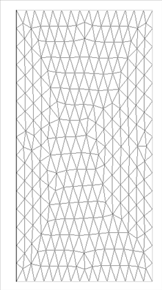
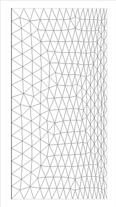
The following two figures illustrate the effect of the Diffusion
Parameter  on the resulting mesh for a translational (piston-type) boundary motion,
when the diffusivity is based on the boundary distance. In this example, an initially
uniformly meshed square domain is deformed by moving the left boundary to the right.
on the resulting mesh for a translational (piston-type) boundary motion,
when the diffusivity is based on the boundary distance. In this example, an initially
uniformly meshed square domain is deformed by moving the left boundary to the right.
For rotational boundary motions, a value of 1.5 for the Diffusion
Parameter  is recommended as a good starting point.
Two different methods are available for the evaluation of the boundary distance
 if boundary-distance-based diffusion is used. By default, Fluent uses the
“standard” boundary distance in Equation 13–3,
which is the normalized distance to the nearest wall boundary; note that none of the other
boundary types (for example, inlets, outlets, symmetry, and periodic boundaries) are
considered. This method is the same as that which is used to evaluate the boundary distance
for turbulence models. An example of this method is shown in Figure 13.20: Effect of Diffusion Parameter of 1 on Interior Node Motion, where only the left and right boundaries are walls.
You have the option of enabling the Generalized Boundary Distance Method
option instead, so that is the normalized distance to the nearest boundary that is not declared as
deforming, regardless of type. Both methods use the largest distance found in all deforming
cell zones to normalize the value.
if boundary-distance-based diffusion is used. By default, Fluent uses the
“standard” boundary distance in Equation 13–3,
which is the normalized distance to the nearest wall boundary; note that none of the other
boundary types (for example, inlets, outlets, symmetry, and periodic boundaries) are
considered. This method is the same as that which is used to evaluate the boundary distance
for turbulence models. An example of this method is shown in Figure 13.20: Effect of Diffusion Parameter of 1 on Interior Node Motion, where only the left and right boundaries are walls.
You have the option of enabling the Generalized Boundary Distance Method
option instead, so that is the normalized distance to the nearest boundary that is not declared as
deforming, regardless of type. Both methods use the largest distance found in all deforming
cell zones to normalize the value.
If the generalized boundary distance is used, an additional scalar equation for the
boundary distance  will be solved as part of the solution of Equation 13–2.
Using cell-volume-based diffusion (Equation 13–4) allows you to control how the boundary motion diffuses into the interior of the domain as a function of cell size. Decreasing the diffusivity in larger cells causes those cells to absorb more of mesh motion and therefore better preserves the cell quality of smaller cells.
You can manipulate the diffusion coefficient  (in Equation 13–3) by adjusting the
Diffusion Parameter in the Mesh Smoothing Parameters Dialog Box (
(in Equation 13–3) by adjusting the
Diffusion Parameter in the Mesh Smoothing Parameters Dialog Box (  ). A value of 0 (the default value) specifies that
  and yields a uniform diffusion of the boundary motion throughout the mesh.
Higher values of
and yields a uniform diffusion of the boundary motion throughout the mesh.
Higher values of  result in larger cells absorbing more of the motion than smaller
cells.
result in larger cells absorbing more of the motion than smaller
cells.
Note that the cell volume used in Equation 13–4 is the local cell volume, normalized by the average cell volume of all deforming cell zones.
Diffusion-based mesh smoothing can be used to update any cell zone whose boundaries are moving or deforming. It is available for all element types, though it is not as robust for polyhedral elements as radial basis function smoothing.
Diffusion-based smoothing is computationally more expensive than spring-based smoothing, but likely results in better mesh quality (especially for non-tetrahedral / non-triangular cell zones, and for polyhedral cells in particular) and generally allows for larger boundary deformations before breaking down.
Similar to spring-based smoothing, diffusion-based mesh smoothing can handle translational boundary deformations much better than rotational motions. Rotational motions are best handled by radial basis function smoothing.
Diffusion-based smoothing is not compatible with the boundary layer smoothing method or the face region remeshing method. For more information about these methods, see Boundary Layer Smoothing Method and Face Region Remeshing Method.
Unlike the radial basis function smoothing method, the diffusion-based smoothing method is not supported when the smoothing zone contains deforming conformal periodic boundaries and/or is a solid that has a moving wall.
For spring-based smoothing, the edges between any two mesh nodes are idealized as a network of interconnected springs. The initial spacings of the edges before any boundary motion constitute the equilibrium state of the mesh. A displacement at a given boundary node will generate a force proportional to the displacement along all the springs connected to the node. Using Hook’s Law, the force on a mesh node can be written as
 | (13–6) |
where  and
and  are the displacements of node
  and its neighbor
  ,
,  is the number of neighboring nodes connected to node
  , and
, and  is the spring constant (or stiffness) between node
  and its neighbor
  . The spring constant for the edge connecting nodes
  and
and  is defined as
 | (13–7) |
where  is the value you enter for Spring Constant Factor in
the Mesh Smoothing Parameters Dialog Box.
is the value you enter for Spring Constant Factor in
the Mesh Smoothing Parameters Dialog Box.
At equilibrium, the net force on a node due to all the springs connected to the node must be zero. This condition results in an iterative equation such that
 | (13–8) |
where  is the iteration number.
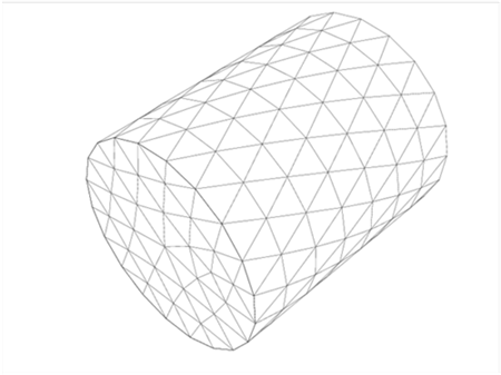
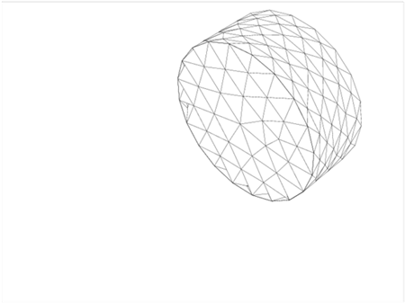
Since displacements are known at the boundaries (after boundary node positions have been updated), Equation 13–8 is solved using a Jacobi sweep on all interior nodes. At convergence, the positions are updated such that
 | (13–9) |
where  and
and  are used to denote the positions at the next time step and the current time
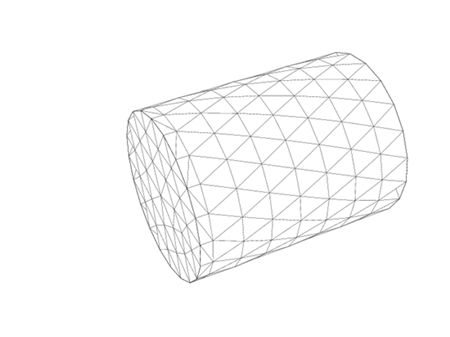
step, respectively. The spring-based smoothing is shown in Figure 13.21: Spring-Based Smoothing on Interior Nodes: Start and Figure 13.22: Spring-Based Smoothing on Interior Nodes: End for a cylindrical
cell zone where one end of the cylinder is moving.
are used to denote the positions at the next time step and the current time
step, respectively. The spring-based smoothing is shown in Figure 13.21: Spring-Based Smoothing on Interior Nodes: Start and Figure 13.22: Spring-Based Smoothing on Interior Nodes: End for a cylindrical
cell zone where one end of the cylinder is moving.
You can control the spring stiffness by adjusting the value of the Spring Constant Factor between 0 and 1. A value of 0 indicates that there is no damping on the springs, and boundary node displacements have more influence on the motion of the interior nodes. A value of 1 imposes the default level of damping on the interior node displacements as determined by solving Equation 13–8.
The effect of the Spring Constant Factor is illustrated in Figure 13.23: Interior Nodes Extend Beyond Boundary (Spring Constant Factor = 1) and Figure 13.24: Interior Nodes Remain Within Boundary (Spring Constant Factor = 0), which show the trailing edge of a NACA-0012 airfoil after a counter-clockwise rotation of 2.3° and the mesh is smoothed using the spring-based smoother but limited to 20 iterations. Degenerate cells (Figure 13.23: Interior Nodes Extend Beyond Boundary (Spring Constant Factor = 1)) are created with the default value of 1 for the Spring Constant Factor, as the interior nodes extend beyond the moving boundary. However, the original mesh distribution (Figure 13.24: Interior Nodes Remain Within Boundary (Spring Constant Factor = 0)) is recovered if the Spring Constant Factor is set to 0 (that is, no damping on the displacement of interior nodes near the airfoil surface).
You can control the solution of Equation 13–8 using the values of Convergence Tolerance and Maximum Number of Iterations. Ansys Fluent solves Equation 13–8 iteratively during each time step until one of the following criteria is met:


You can use the spring-based smoothing method to update any cell or face zone whose boundary is moving or deforming.
For non-tetrahedral cell zones (non-triangular in 2D), the spring-based method can be used when the following conditions are met:
The boundary of the cell zone moves predominantly in one direction (that is, no excessive anisotropic stretching or compression of the cell zone).
The motion is predominantly normal to the boundary zone.
If these conditions are not met, the resulting cells may have high skewness values, since not all possible combinations of node pairs in non-tetrahedral cells (or non-triangular in 2D) are idealized as springs. Polyhedral cells are particularly likely to become highly skewed with spring-based smoothing (regardless of whether the previous conditions are met), and so the radial basis function smoothing method is generally recommended for polyhedra (see Radial Basis Function Smoothing).
By default, spring-based smoothing is enabled for all cell zones. This is reflected in the Mesh Smoothing Parameters Dialog Box, where All is selected from the Elements list. If you want to disable spring-based smoothing for cell zones that are not entirely composed of either tetrahedral or triangular cells, you can do that by selecting Tet in Tet Zones in 3D (or Tri in Tri Zones in 2D).
If you have mixed element zones and you do not want spring-based smoothing on all element types, you can enable spring-based smoothing on only the tetrahedral or triangular cells by selecting Tet in Mixed Zones in 3D (or Tri in Mixed Zones in 2D). Selection of smoothing elements in the Mesh Smoothing Parameters Dialog Box applies by default to all cell zones that undergo spring-based smoothing. In order to have more precise control, it is possible to overwrite this global selection on individual dynamic cell zones (see Deforming Motion). This gives, for example, the flexibility to suppress smoothing in zones where dynamic layering (see Dynamic Layering) is used and allows at the same time smoothing of non-simplex (that is not tetrahedral or triangular) elements in other zones.
Unlike the radial basis function smoothing method, the spring-based smoothing method is not supported when the smoothing zone contains deforming conformal periodic boundaries and/or is a solid that has a moving wall.
With mesh smoothing based on the linearly elastic solid model, the mesh motion is governed by the following set of equations.
 | (13–11) |
where  is the stress tensor,
  is the strain tensor, and
  is the mesh displacement. For the solution of Equation 13–11 only the ratio between the shear modulus,
 , and Lamé’s first parameter,
  , matters. This ratio is parameterized through Poisson’s ratio
(
, matters. This ratio is parameterized through Poisson’s ratio
( ):
):
 | (13–12) |
You define this property through the Poisson's Ratio field in the Mesh Smoothing Parameters Dialog Box. Note that the linearly elastic solid mesh smoothing model supports constant material properties only. The permissible range for Poisson's Ratio is between -1.0 and 0.5.
The boundary conditions for Equation 13–11 are obtained from the user-prescribed or computed (in the case of six DOF motion) boundary deformations. These imposed deformations are transferred into the interior of the deforming mesh as if the mesh was a linearly elastic solid with the given material properties. On deforming boundaries you can either specify a geometry along which the mesh can slide, or leave the geometry unspecified. If a geometry is specified for the deforming boundary, then the boundary conditions are such that the deformation normal to the boundary vanishes and the stress tangential to the boundary is zero. If the geometry of the deforming boundary is unspecified, then the deforming boundary can also deform in the normal direction and the boundary conditions are such that the traction is zero in all directions. See Deforming Motion for details of how to specify geometry on deforming zones.
The linear system in Equation 13–11 is solved using a finite element discretization and the mesh displacements for the interior and deforming boundary nodes are obtained directly at the nodes. The accuracy to which the linear system is solved can be controlled by the Maximum Number of Iterations and the Relative Convergence Tolerance.
You can specify the solution method used by the linear solver for the linearly elastic solid mesh smoothing calculations. By default, the CG (conjugate gradient) method is selected from the AMG Stabilization drop-down list. This method should be faster in this context than the other available methods, as it takes advantage of the symmetry of the matrix used in the linear systems of equations of finite-element-based mesh smoothing. If divergence is detected with CG, then the generalized minimal residual (GMRES) method will be used for an iteration as a fallback, and you will be informed in the console that a finite-element-based mesh smoothing coupled equation is being stabilized to enhance linear solver robustness. In rare cases, the CG method may result in the generation of negative volume cells; you may be able to avoid this by increasing the Maximum Number of Iterations from the default of 50 to a value in the range of 200–500.
If the CG method continues to generate negative volume cells with a higher number of inner iterations or if you repeatedly see console messages that say the GMRES fallback is being used, it is recommended that you select GMRES from the AMG Stabilization drop-down list. Note that the GMRES method is more robust than the CG method, especially for high-aspect-ratio meshes; but it is also more demanding in terms of memory usage and solver time.
Note that this drop-down list also allows you to select the BCGSTAB (bi-conjugate gradient stabilized) method; like the CG method, BCGSTAB falls back to the GMRES method for an iteration when divergence is detected.
You can enable printing of smoothing residuals in the console by entering 1 for the Verbosity.
For simulations with periodic or quasi-periodic motion, you can improve the mesh quality consistency by specifying that the linearly elastic solid mesh smoothing uses a reference position, as described in Smoothing from a Reference Position.
Most of the properties and limitations discussed for diffusion-based smoothing (Applicability of the Diffusion-Based Smoothing Method) also apply to the linearly elastic solid model, particularly the mesh quality degradation for rotational motions. The linearly elastic solid model is computationally more expensive than diffusion-based smoothing, but for some meshes and mesh motions preserves the mesh quality better.
The current implementation with constant material properties can be a limitation compared with diffusion-based smoothing with non-uniform diffusivity. In cases with rotational boundary motion and sharp corners it may be advantageous to use radial basis function smoothing, or perhaps diffusion-based smoothing with boundary-distance-dependent diffusivity.
The linearly elastic solid smoothing method provides you the option to leave the geometry of deforming face zones unspecified. This option is not available for any other smoothing method except for the radial basis function method.
The linearly elastic solid smoothing method supports triangular and quadrilateral elements in 2D and tetrahedral, hexahedral, wedge, and pyramid cells in 3D. It cannot be applied if the deforming cell zone contains polyhedral cells or hanging nodes. In such cases radial basis function smoothing is recommended.
Linearly elastic solid smoothing is not compatible with the boundary layer smoothing method or the face region remeshing method. For more information about these methods, see Boundary Layer Smoothing Method and Face Region Remeshing Method.
Unlike the radial basis function smoothing method, the linearly elastic solid smoothing method is not supported when the smoothing zone contains deforming conformal periodic boundaries and/or is a solid that has a moving wall.
When the smoothing is based on a radial basis function interpolation, Fluent solves for a displacement field that satisfies the displacements at boundaries with prescribed motion, and then interpolates the displacements onto all other nodes in the interior and at the deforming boundaries. As with the other available smoothing methods, deforming boundaries are boundaries where the nodes are allowed to slide tangentially.
Radial basis function smoothing has the following advantages:
Compared to the other available smoothing methods, it is particularly well suited for motions that undergo rotation. On average, more rotational motion can be absorbed by the mesh with radial basis function smoothing before the mesh quality degenerates.
Unlike linearly elastic solid based smoothing, it is available for adapted meshes with hanging nodes or polyhedra elements.
Unlike diffusion smoothing, it is robust for polyhedral elements.
It is the only smoothing method that is supported when:
the smoothing zone contains deforming conformal periodic boundaries.
the smoothing zone is a solid that has a moving wall, as may be the case in a simulation that models ablation or erosion / accretion (see Thermal Conditions for Two-Sided Walls and Particle Erosion Coupled with Dynamic Meshes, respectively). Note that the ablation or erosion / accretion must be set up on the fluid side of the coupled wall.
On deforming boundaries, you can either specify a geometry (such as a plane, cylinder, and so on) along which the mesh can slide, or leave the geometry unspecified so that the nodes are allowed to move in any direction. See Deforming Motion for details of how to define the geometry for deforming zones. The ability to leave the geometry of deforming face zones unspecified is not available for any other smoothing method except for the radial basis function smoothing method and the linearly elastic solid smoothing method. Note that if you have a non-conformal interface where both of the interface boundaries are defined as deforming dynamic zones with unspecified geometry, then Fluent will ensure that the two interface zones stay connected (by projecting one of the interface zones onto the other); such behavior is only supported with radial basis function smoothing, and then only if the same cell zone is on either side of the non-conformal interface.
Advanced settings are available for radial basis function smoothing in the Mesh Smoothing Parameters Dialog Box. The accuracy to which the displacement field is solved can be controlled by the Relative Convergence Tolerance: if the smoothing produces negative volume cells, you can decrease this value to try to address the problem; if the solution is running well, you can increase the value to speed up the calculation. You can also set the Verbosity to 1 if you want to print the absolute tolerance computed (based on your specified relative tolerance) in the console during the calculation. If you want to limit the amount of the domain that is smoothed to only those cells that are close to the moving boundary zone(s), you can enable the Local Smoothing option (for details, see Local Smoothing with the Radial Basis Function Smoothing Method). Finally, you can specify that the smoothing uses a reference position (as described in Smoothing from a Reference Position), which can improve mesh quality consistency when performing many cycles of periodic or quasi-periodic motion for stationary or moving meshes.
If you want to smooth the entire mesh but would like to take advantage of the boundary layer smoothing that is done as part of the Local Smoothing option (and hence retain the shape of the boundary layers as much as possible), you can make sure that the Local Smoothing option is disabled and use the following text command:
define → dynamic →
controls → smoothing-parameters
→ smooth-boundary-layers-with-adjacent-zone?
Note the following limitations:
The performance of radial basis function smoothing does not scale as well as the other smoothing methods when running distributed memory on a cluster.
Radial basis function smoothing is not compatible with the boundary layer smoothing method. For more information about this method, see Boundary Layer Smoothing Method.
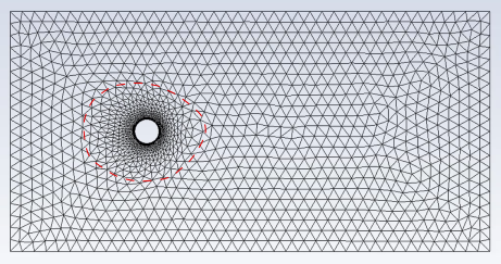
As mentioned in the previous section, you can enable the Local Smoothing option in the Mesh Smoothing Parameters Dialog Box when using the radial basis function smoothing method, so that only the portion of the mesh adjacent to the moving boundary zone is smoothed. This ensures that the mesh away from the moving boundary remains undisturbed by the smoothing, and decreases the computational time required for smoothing. The following figure provides an example of such local smoothing: the circular boundary zone is moving to the right, and only those cells within the red dotted line are smoothed, while the rest of the domain is unaffected.
Note: Depending on the amplitude of motion, it might be necessary to enable remeshing along with the local smoothing, as the motion is now absorbed in a smaller region. For details, see Remeshing.
If there are boundary layers adjacent to the moving zone, they are smoothed before and independently of the local smoothing region, ensuring that they retain their shape as much as possible. The portion of the mesh smoothed by the local smoothing is then evaluated starting from the edge of the boundary layers. When identifying which cells are boundary layers, Fluent searches for prismatic cells (that is, hexahedral cells or wedge or polyhedral cells that have the same number of nodes on the top and bottom faces relative to the boundary normal) that are in layers adjacent to a boundary zone.
When the mesh smoothing is based on diffusion, the linearly elastic solid model, or a radial basis function interpolation, you have the option of specifying that the smoothing uses a reference position. This can be helpful when performing many cycles of periodic or quasi-periodic motion for stationary or moving meshes; for example, turbomachinery rotors with blade flutter. When you ensure that the smoothing is always done from the same reference position, the mesh quality may remain more consistent from cycle to cycle.
To use this feature, enable the Smoothing From Reference Position option in the Mesh Smoothing Parameters Dialog Box. Note this option is enabled by default during the calculation if the case includes a cell zone that has Frame Motion or Mesh Motion enabled with a nonzero rotational velocity and that is also defined as a deforming dynamic mesh zone. This option is not available if the Layering and/or Remeshing options are enabled in the Dynamic Mesh task page, or if automatic adaption criteria is activated in the Manage Adaption Criteria dialog box.
The reference position is saved the first time you perform smoothing after enabling this
option. It is recommended that you do not save your case / data files in the legacy format
(that is, with the file/cff-file? text command set to
no): the reference position is not saved in this format, and so
restarting from a .cas file will imply that a different reference
position is used after restart. This still provides the benefit of consistent quality, but the
resulting meshes might be slightly different from a continuous run. The impact of such slight
mesh changes on the solution results will be small, except for cases with a high degree of
mesh dependence; if you must use a legacy case file, it is recommended that you evaluate the
original mesh to ensure that it is suitable for the problem.
Laplacian smoothing is the most commonly used and the simplest mesh smoothing method. This method adjusts the location of each mesh vertex to the geometric center of its neighboring vertices. This method is computationally inexpensive but it does not guarantee an improvement on mesh quality, since repositioning a vertex by Laplacian smoothing can result in poor quality elements. To overcome this problem, Ansys Fluent only relocates the vertex to the geometric center of its neighboring vertices if and only if there is an improvement in the mesh quality (that is, the skewness has been improved).
This improved Laplacian smoothing can be enabled on deforming boundaries only (that is, the zone with triangular elements in 3D and zones with linear elements in 2D). The computation of the node positions works as follows:
 | (13–13) |
where  is the averaged node position of node
  at iteration
  ,
,  is the node position of neighbor node of
  at iteration
  , and
, and  is the number nodes neighboring node
  . The new node position
  is then computed as follows:
 | (13–14) |
where  is the Laplace node relaxation factor.
This update only happens if the maximum skewness of all faces adjacent to  is improved in comparison to
  .
.
For details on applying Laplacian smoothing to either a cell zone (with 2.5D remeshing) or a face zone, see Smoothing Methods or Deforming Motion, respectively.
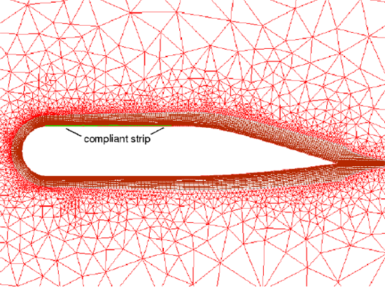
The boundary layer smoothing method is used to deform the boundary layer mesh during a moving-deforming mesh simulation. For cases that apply mesh motion (either Rigid Body or User-Defined) to a face zone with adjacent boundary layers, the boundary layers can be made to deform accordingly by enabling Deform Adjacent Boundary Layer with Zone for the face zone in the Dynamic Mesh Zones Dialog Box. With boundary layer smoothing enabled, the nodal coordinates of each cell in the boundary layer zone are updated with the same displacement vector as the corresponding nodes on the underlying face zone. The boundary layer smoothing method can be applied to boundary layer zones of all mesh types (that is, wedges and hexahedra in 3D, quadrilaterals in 2D).
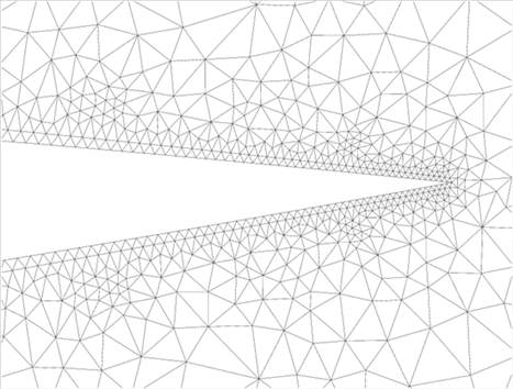
Consider the example below, where a UDF of the form
DEFINE_GRID_MOTION provides the moving-deforming mesh model with the
locations of the nodes located on the compliant strip on an idealized airfoil. The node motion
varies sinusoidally in time and space (compare Figure 13.26: The Undeformed Mesh with Figure 13.27: The Deformed Mesh).
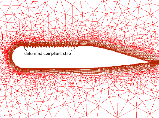
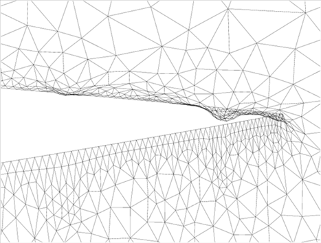
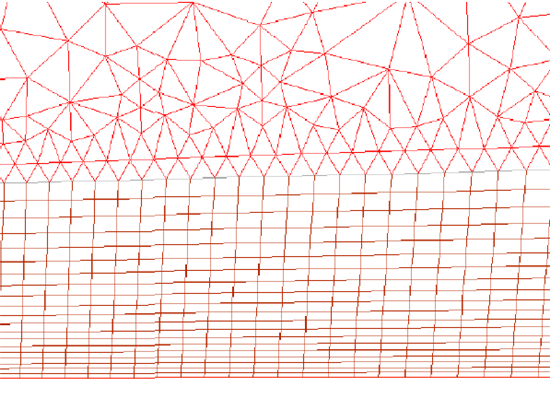
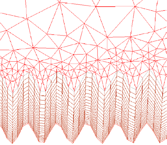
As a result of the boundary layer smoothing, the cells adjacent to the deforming wall are also deformed in order to preserve the quality of boundary layer zone. If you compare Figure 13.28: Zooming into the Undeformed Compliant Strip with Figure 13.29: Zooming into the Deformed Compliant Strip with Boundary Layer Smoothing Applied, you can see how the boundary layer cells have been deformed according to the motion of the nodes on the compliant strip.
Typically, the boundary layer smoothing method preserves the height of the boundary layer cells adjacent to the deformed face zone. However, note that this approach is primarily intended for translational motion. If the faces undergo substantial rotation, the boundary layer cells may become skewed. See Smoothing Methods and Specifying Boundary Layer Deformation Smoothing for details about enabling smoothing and defining a moving and deforming boundary layer, respectively. Note that boundary layer smoothing is compatible with spring-based smoothing only. It cannot be used with diffusion-based smoothing, linearly elastic solid smoothing, or radial basis function smoothing. Also note that the boundary layer smoothing method will work whether or not you have segregated the boundary layer elements into a separate cell zone.
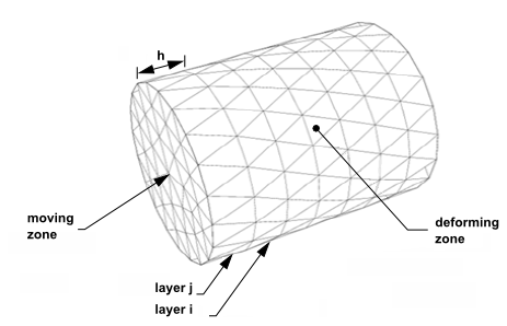
In prismatic (polyhedral, hexahedral, and/or wedge in 3D, or quadrilateral in 2D) mesh
zones, you can use dynamic layering to add or remove layers of cells adjacent to a moving
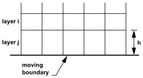
boundary, based on the height of the layer adjacent to the moving surface. The dynamic mesh
model in Ansys Fluent allows you to specify an ideal layer height on each moving boundary. The
layer of cells adjacent to the moving boundary (layer  in Figure 13.30: Dynamic Layering) is split or merged
with the layer of cells next to it (layer
in Figure 13.30: Dynamic Layering) is split or merged
with the layer of cells next to it (layer  in Figure 13.30: Dynamic Layering) based on the height
(
in Figure 13.30: Dynamic Layering) based on the height
( ) of the cells in layer
  .
.
If the cells in layer  are expanding, the cell heights are allowed to increase until
 | (13–15) |
where  is the minimum cell height of cell layer
  ,
,  is the ideal cell height, and
  is the layer split factor. Note that Ansys Fluent allows you to define
 as either a constant value or a value that varies as a function of time or
crank angle. When the condition in Equation 13–15 is met,
the cells are split based on the specified layering option. This option can be height based or
ratio based.
as either a constant value or a value that varies as a function of time or
crank angle. When the condition in Equation 13–15 is met,
the cells are split based on the specified layering option. This option can be height based or
ratio based.
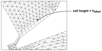
With the height-based option, the cells are split to create a layer of cells with constant
height  and a layer of cells of height
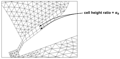
  . With the ratio-based option the cells are split such that, locally, the
ratio of the new cell heights to old cell heights is exactly
. With the ratio-based option the cells are split such that, locally, the
ratio of the new cell heights to old cell heights is exactly  everywhere. Figure 13.31: Results of Splitting Layer with the Height-Based Option and Figure 13.32: Results of Splitting Layer with the Ratio-Based Option show the result of splitting a layer of cells above a
valve geometry using the height-based and ratio-based option.
everywhere. Figure 13.31: Results of Splitting Layer with the Height-Based Option and Figure 13.32: Results of Splitting Layer with the Ratio-Based Option show the result of splitting a layer of cells above a
valve geometry using the height-based and ratio-based option.
If the cells in layer  are being compressed, they can be compressed until
 | (13–16) |
where  is the layer collapse factor. When this condition is met, the compressed
layer of cells is merged into the layer of cells above the compressed layer in Figure 13.30: Dynamic Layering; that is, the cells in layer
is the layer collapse factor. When this condition is met, the compressed
layer of cells is merged into the layer of cells above the compressed layer in Figure 13.30: Dynamic Layering; that is, the cells in layer  are merged with those in layer
  .
.
To enable dynamic layering, enable the Layering option under Mesh Methods in the Dynamic Mesh Task Page (Figure 13.33: The Layering Tab in the Mesh Method Settings Dialog Box). The layering control is specified in the Layering tab, which can be displayed by clicking .
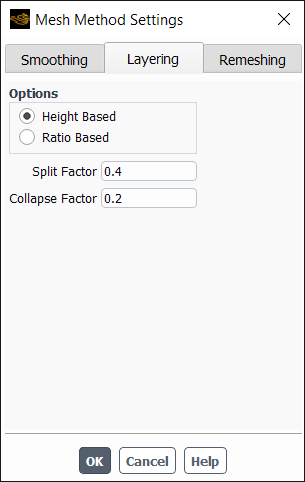
You can control how a cell layer is split by specifying either Height Based or Ratio Based under Options. Note that for Height Based, the height of the cells in a particular new layer will be constant, but you can choose to have this height vary from layer to layer as a function of time or crank angle when you specify the Cell Height in the Dynamic Mesh Zones dialog box (see Specifying the Motion of Dynamic Zones for further details).
The Split Factor and Collapse Factor
( in Equation 13–15 and
  in Equation 13–16, respectively) are
the factors that determine when a layer of prismatic cells (polyhedra, hexahedra, or wedges in
3D, or quadrilaterals in 2D) that is next to a moving boundary is split or merged with the
adjacent cell layer, respectively.
in Equation 13–16, respectively) are
the factors that determine when a layer of prismatic cells (polyhedra, hexahedra, or wedges in
3D, or quadrilaterals in 2D) that is next to a moving boundary is split or merged with the
adjacent cell layer, respectively.
You can use the dynamic layering method to split or merge cells adjacent to any moving boundary provided the following conditions are met:
All cells adjacent to the moving face zone are prismatic and either polyhedra, hexahedra, or wedges (quadrilaterals in 2D), even though the cell zone may contain mixed cell shapes.
The cell layers must be completely bounded by one-sided face zones, except when sliding interfaces are used (see Applicability of the Face Region Remeshing Method).
Note that you cannot use the dynamic layering method in conjunction with adaption in almost all cases. For more information on the available adaption methods, see Hanging Node Adaption and Polyhedral Unstructured Mesh Adaption in the Theory Guide.
If the moving boundary is an internal zone, cells on both sides (possibly with different ideal cell layer heights) of the internal zone are considered for dynamic layering.
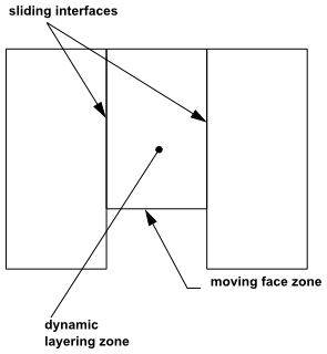
If you want to use dynamic layering on cells adjacent to a moving wall that do not span from boundary to boundary, you must separate those cells that are involved in the dynamic layering and use the sliding interfaces capability in Ansys Fluent to transition from the deforming cells to the adjacent non-deforming cells (see Figure 13.34: Use of Sliding Interfaces to Transition Between Adjacent Cell Zones and the Dynamic Layering Cell Zone). For a moving interior face, the zones must be separated such that they are either expanding or collapsing on the same side. No one zone can consist of both expanding and collapsing layers.
Figure 13.34: Use of Sliding Interfaces to Transition Between Adjacent Cell Zones and the Dynamic Layering Cell Zone
When the boundary displacement is large compared to the local cell sizes, the cell quality can deteriorate or the cells can become degenerate if only mesh smoothing is used. This will invalidate the mesh (for example, result in negative cell volumes) and consequently, will lead to convergence problems when the solution is updated to the next time step.
To circumvent this problem, Ansys Fluent can agglomerate cells that violate the skewness or size criteria and locally remesh the agglomerated cells or faces. If the new cells or faces satisfy the skewness criterion, the mesh is locally updated with the new cells (with the solution interpolated from the old cells). Otherwise, the new cells are discarded and the old cells are retained.
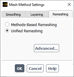
When defining the remeshing settings for your dynamic zones, it is recommended that you use unified remeshing (the default), which applies an algorithm that combines aspects of a variety of remeshing methods and by default attempts to maintain the initial mesh size distribution even as the mesh moves. This simplifies the setup and can provide increased robustness, especially for parallel simulations. It should be noted that such unified remeshing is applied to triangular or tetrahedral cells and can produce wedge cells in 3D boundary layer meshes. As an alternative, you can use methods-based remeshing, which allows you to selectively enable the following options, each of which is suitable for particular kinds of cell types:
The local cell remeshing method only affects triangular and tetrahedral cell types in the mesh (that is, in mixed cell zones the non-triangular/tetrahedral cells are skipped).
The local face remeshing method is available in 3D only and can remesh tetrahedral cells and wedge cells in boundary layer meshes.
The zone remeshing method replaces all cell types with triangular and tetrahedral cells (in 2D and 3D domains, respectively), and can remesh and produce wedge cells in 3D boundary layer meshes.
The face region remeshing method is applied to triangular cells in 2D, and tetrahedral cells in 3D. In 3D domains, the face region remeshing method can also remesh and produce wedge cells in 3D boundary layer meshes.
The 2.5D remeshing method only works on hexagonal meshes or wedge cells extruded from triangular surface elements.
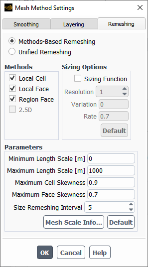
To apply remeshing, enable the Remeshing option under Mesh Methods in the Dynamic Mesh Task Page (Figure 13.13: The Dynamic Mesh Task Page). Click the button to open the Mesh Method Settings dialog box, where you can select either Methods-Based Remeshing or Unified Remeshing in the Remeshing tab (Figure 13.35: The Remeshing Tab in the Mesh Method Settings Dialog Box for Methods-Based Remeshing) and revise the options / parameters or the advanced settings.
For Methods-Based Remeshing, you can view the vital statistics of your mesh by clicking the button at the bottom of the Mesh Method Settings Dialog Box. This button opens the Mesh Scale Info Dialog Box, where you can view the minimum and maximum length scale values, as well as the maximum cell and face skewness values.
For details, see the following sections:
When Methods-Based Remeshing is selected in the Remeshing tab of the Mesh Method Settings dialog box, you can selectively enable the following methods:
Using the local remeshing method (that is, local cell remeshing, with or without local face remeshing), Ansys Fluent marks cells based on cell skewness and minimum and maximum length scales as well as an optional sizing function.
Ansys Fluent evaluates each cell and marks it for remeshing if it meets one or more of the following criteria:
It has a skewness that is greater than a specified maximum skewness.
It is smaller than a specified minimum length scale.
It is larger than a specified maximum length scale.
Its height does not meet the specified length scale (at moving face zones, for example, above a moving piston).
If local remeshing is not able to reduce the maximum cell skewness sufficiently, then the cell zone remeshing method is used to automatically remesh all of the cells in the cell zone, as well as the faces of all adjacent deforming dynamic face zones (see Cell Zone Remeshing Method for details). The maximum allowable cell skewness is set to be 0.98 by default. The cell zone remeshing method gives the mesher more flexibility to create a new mesh of better quality than the local cell remeshing method. The automatic remeshing of cell zones can be disabled using the following text command:
define → dynamic-mesh
→ controls →
remeshing-parameter →
zone-remeshing
As previously mentioned, in local cell remeshing, Ansys Fluent agglomerates cells based on skewness, size, and height (adjacent moving face zones) prior to the movement of the boundary. The size criteria are specified with Minimum Length Scale and Maximum Length Scale. Cells with length scales below the minimum length scale and above the maximum length scale are marked for remeshing. The value of Maximum Cell Skewness indicates the desired skewness of the mesh. By default, the Maximum Cell Skewness is set to 0.9 for 3D simulations and 0.7 for 2D simulations. Cells with skewness above the maximum skewness are marked for remeshing.
The marking of cells based on skewness is done at every time step when the local remeshing method is enabled. However, marking based on size and height is performed between the specified Size Remeshing Interval since the change in cell size distribution is typically small over one time step.
Note that you should edit the fields in the Parameters group box, as the initial values are unlikely to produce your desired outcome. Clicking will define values that are based on your particular mesh and that should represent a reasonable starting point, and you can then adjust them as needed. After you click the button, it will then change to be a button, which can be used to return to the prior values.
By default, Ansys Fluent replaces the agglomerated cells only if the quality of the remeshed cells has improved.
Note that you cannot use the local cell remeshing method in conjunction with adaption. For more information on the available adaption methods, see Hanging Node Adaption and Polyhedral Unstructured Mesh Adaption in the Theory Guide.
The local face remeshing method only applies to 3D geometries. You can apply this method to the boundaries of deforming or user-defined zone types, so that Ansys Fluent will mark faces (and adjacent cells) based on the face skewness, and then remesh them.
Local face remeshing also allows the remeshing of wedge cells in boundary layers at those boundaries. The detection of boundary layers (as well as the wedge element height distribution and number of layers) is automatic and does not require your input.
To apply local face remeshing, perform the following steps:
Enable the Local Face option in the Remeshing tab of the Mesh Method Settings Dialog Box, and set the Maximum Face Skewness to an appropriate global value.
For each deforming or user-defined boundary zone on which you want local face remeshing applied, enable the Local option in the Meshing Options tab of the Dynamic Mesh Zones Dialog Box. You can also revise the Maximum Skewness in this tab if you don't want to use the global setting for a particular zone. Note that for deforming zones, the Remeshing option must be enabled—which is the default condition—in order to access the Local option, and the Global Settings option must be disabled to revise the Maximum Skewness. For further details on the zone setup, see Deforming Motion and/or User-Defined Motion.
When you enable local face remeshing for a boundary, the faces can be remeshed only if the following conditions are met:
The faces are triangular.
The agglomerated faces do not span multiple zones or feature edges.
Note that you cannot use the local face remeshing method in conjunction with adaption. For more information on the available adaption methods, see Hanging Node Adaption and Polyhedral Unstructured Mesh Adaption in the Theory Guide.
Instead of marking cells based on minimum and maximum length scales, Ansys Fluent also marks cells based on the size distribution generated by the sizing function if the Sizing Function option is enabled.
Cells can be marked using sizing functions only with the following remeshing methods:
local cell remeshing
2.5D surface remeshing (as described in 2.5D Surface Remeshing Method)
Figure 13.38: Mesh at the End of a Dynamic Mesh Simulation With Sizing Functions demonstrates the advantages of using sizing functions for local remeshing.
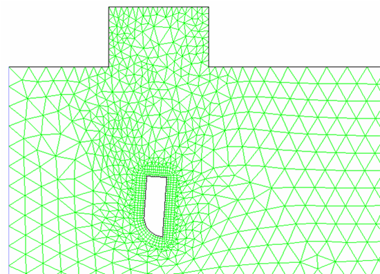
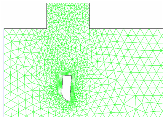
In determining the sizing function, Ansys Fluent draws a bounding box around the zone that is approximately twice the size of the zone, and locates the shortest feature length within each fluid zone. Ansys Fluent then subdivides the bounding box based on the shortest feature length and the sizing function Resolution that you specify. This allows Ansys Fluent to create a background mesh.
You control the resolution of the background mesh and a background mesh is created for each fluid zone. The shortest feature length is determined by shrinking a second box around the object, and then selecting the shortest edge on that box. The sizing function is evaluated at the vertex of each individual background mesh.
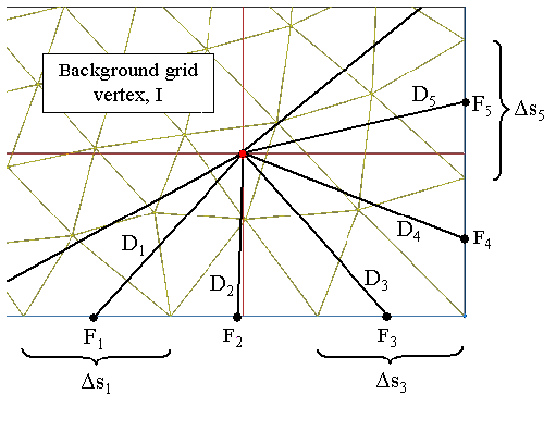
As seen in Figure 13.39: Sizing Function Determination at Background Mesh Vertex I, the local value of the
sizing function  is defined by
 | (13–17) |
where  is the distance from vertex
  on the background mesh to the centroid of boundary cell
  and
and  is the mesh size (length) of boundary cell
  .
.
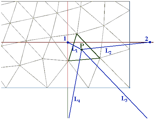
The sizing function is then smoothed using Laplacian smoothing. Ansys Fluent then
interpolates the value of the sizing function by calculating the distance  from a given cell centroid
  to the background mesh vertices that surround the cell (see Figure 13.40: Interpolating the Value of the Sizing Function). The intermediate value of the sizing
function
to the background mesh vertices that surround the cell (see Figure 13.40: Interpolating the Value of the Sizing Function). The intermediate value of the sizing
function  at the centroid is computed from
 | (13–18) |
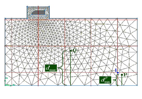
Next, a single point  is located within the domain (see Figure 13.41: Determining the Normalized Distance) that has the largest distance
  to the nearest boundary to it. The normalized distance
  for the given centroid
  is given by
 | (13–19) |
Using the parameters  and
and  (the sizing function Variation and the sizing
function Rate, respectively), you can write the final value
(the sizing function Variation and the sizing
function Rate, respectively), you can write the final value
 of the sizing function at point
  as
as
 | (13–20) |
where  is the intermediate value of the sizing function at the cell
centroid.
is the intermediate value of the sizing function at the cell
centroid.
Note that  is the sizing function variation. Positive values
mean that the cell size increases as you move away from the boundary. Since the maximum
value of
is the sizing function variation. Positive values
mean that the cell size increases as you move away from the boundary. Since the maximum
value of  is one, the maximum cell size becomes
 | (13–21) |
therefore,  is really a measure of the maximum cell size.
The factor  is computed from
 | (13–22) |
 | (13–23) |
You can use sizing function Variation (or  ) to control how large or small an interior cell can be with respect to its
closest boundary cell.
) to control how large or small an interior cell can be with respect to its
closest boundary cell.  ranges from
  to
to  , an
, an  value of 0.5 indicates that the interior cell size can be, at most, 1.5
the size of the closest boundary cell. Conversely, an
value of 0.5 indicates that the interior cell size can be, at most, 1.5
the size of the closest boundary cell. Conversely, an  value of
  indicates that the cell size interior of the boundary can be half of that
at the closest boundary cell. A value of 0 indicates a constant size distribution away from
the boundary.
indicates that the cell size interior of the boundary can be half of that
at the closest boundary cell. A value of 0 indicates a constant size distribution away from
the boundary.
You can use the sizing function Rate (or  ) to control how rapidly the cell size varies from the boundary. The value
of
) to control how rapidly the cell size varies from the boundary. The value
of  should be specified such that
  . A positive value indicates a slower transition from the boundary to the
specified sizing function Variation value. Conversely, a negative value
indicates a faster transition from the boundary to the sizing function
Variation value. A value of 0 indicates a linear variation of cell size
away from the boundary.
. A positive value indicates a slower transition from the boundary to the
specified sizing function Variation value. Conversely, a negative value
indicates a faster transition from the boundary to the sizing function
Variation value. A value of 0 indicates a linear variation of cell size
away from the boundary.
You can also control the Resolution of the sizing function. This
determines the size of the background bins used to evaluate the size distribution with
respect to the shortest feature length of the current mesh. By default, the sizing function
Resolution is 3 in 2D problems, and
1 in 3D problems.
Note that if you edit the Resolution, Variation, and/or Rate, clicking will return these fields to the default values based on the current mesh. The button will then change to be a button, which can be used to return to the prior values.
In summary, the sizing function is a distance-weighted average of all mesh sizes on all boundary faces (both stationary and moving boundaries). The sizing function is based on the sizes of the boundary cells, with the size computed from the cell volume by assuming a perfect (equilateral) triangle in 2D and a perfect tetrahedron in 3D. You can control the size distribution by specifying the sizing function Variation and the sizing function Rate. If you have enabled the Sizing Function option, Ansys Fluent will agglomerate a cell if
 | (13–24) |
where  is a factor defined by Equation 13–22
and Equation 13–23.
is a factor defined by Equation 13–22
and Equation 13–23.
Note that the sizing function is only used for marking cells before remeshing. The sizing function is not used to govern the size of the cell during remeshing.
For steady-state applications (see Steady-State Dynamic Mesh Applications), you can instruct Ansys Fluent to perform a second round of cell marking and agglomeration after the boundary has moved, based on skewness criteria. The intent is to further improve the mesh quality through additional local remeshing. This optional feature works in conjunction with the Mesh Method Settings dialog box (Figure 13.35: The Remeshing Tab in the Mesh Method Settings Dialog Box for Methods-Based Remeshing), and operates according to the skewness parameters you set in this dialog box. The sizing function parameters are not considered during this additional remeshing. Note that enabling this option will increase the time required to update the mesh during the solution.
Note: If you want to employ additional local remeshing, first make sure that you have enabled the Remeshing option in the Dynamic Mesh Task Page.
To enable the additional round of local remeshing, use the following text command:
define → dynamic-mesh
→ controls →
remeshing-parameter →
remeshing-after-moving?
The cell zone remeshing method allows for the remeshing of the complete cell zone, and provides the option to also remesh the faces of all adjacent deforming dynamic face zones. This remeshing method is enabled by default when local cell remeshing is enabled, and is performed automatically if the local cell remeshing does not produce an acceptable mesh (see Local Remeshing Method for the acceptability criteria). Cell zone remeshing can also be manually invoked, using the following text command:
define → dynamic-mesh
→ actions →
remesh-cell-zone
The cell zone remeshing method is available for triangular cells in 2D meshes and
tetrahedral cells in 3D meshes. For 3D meshes, the method also allows the remeshing of wedge
cells in boundary layers. The detection of the boundary layers (as well as the wedge element
height distribution and number of layers) is automatically performed by default, and allows
for different layer parameters on each boundary zone. You can manually specify the parameters
by entering nonzero values for first height, growth rate, and number of layers via the text
commands available in the
define/dynamic-mesh/controls/remeshing-parameters/prism-layer-parameters
menu, although generally it is not necessary to do this. When you enter them manually, the
boundary layer parameters are global: they apply to every prism layer detected in the
remeshing zone.
Note that it is necessary to enable the dynamic mesh model and the remeshing method in order to attain access to the prism layer controls, even if the cell zone is remeshed manually and not as part of a dynamic mesh update.
The face region remeshing method allows for the remeshing of those triangular faces (in 3D meshes) and linear faces (in 2D meshes) that are on a deforming face zone and adjacent to a moving face zone (see layer j in Figure 13.42: Expanding Cylinder Before Region Face Remeshing). Ansys Fluent marks the faces based on minimum and maximum length scales, and then remeshes the faces and the associated cells to produce a very regular mesh on the deforming boundary. Although primarily designed for in-cylinder type configurations, where the remeshing region is located where cylinder walls meet the moving piston, face region remeshing can be used for all applications where a moving dynamic zone abuts deforming dynamic face zones.
For 3D simulations, Ansys Fluent allows face region remeshing with symmetric boundary conditions and across multiple face zones. The remeshing can preserve features not only between the different deforming face zones, but also within a face zone. For more information on feature preservation, see Feature Detection. Ansys Fluent also allows face region remeshing of tetrahedral cell zones that contain wedge cells in boundary layers, as described in the section that follows.
To begin marking the faces for face region remeshing, Ansys Fluent identifies the nodes at the intersection of a moving dynamic zone and the adjacent deforming zones. Ansys Fluent then analyzes the height of the faces on the deforming zones that are in the range of the identified nodes, and then remeshes the faces depending on the specified maximum or minimum length scale.
Consider the simple tetrahedral mesh of a cylinder that has a moving end wall (see Figure 13.42: Expanding Cylinder Before Region Face Remeshing). The faces that are subject to remeshing are in layer j of the side wall. If the faces in layer j are expanding, the expansion continues until the height h reaches the maximum length scale, and then the layer is remeshed to form 2 layers of elements (see Figure 13.43: Expanding Cylinder After Region Face Remeshing). Conversely, if the faces of layer j are contracting, the contraction continues until h reaches the minimum length scale, and then layer j and the neighboring layer of faces (layer i) on the deforming zone are remeshed to form a single layer.
In 3D simulations, the face region remeshing method can be applied on meshes that have wedge cells along the deforming face zones. When remeshing the faces on the deforming face zones, the associated wedge cells are remeshed as well. The layer parameters are based on the existing mesh by default; you have the option of manually setting these parameters, as described later in this section.
If the motion of the face zone is large compared to the height of the adjacent deforming face zones, it is recommended that you decompose the mesh volume in such a way as to create a dynamic cell zone that moves as a rigid body in between the moving face zone and the deforming dynamic cell zone on which face region remeshing is applied. Consider Figure 13.44: Volume Decomposition for Prism Layers, which displays only half of an in-cylinder mesh. The rigidly moving cell zone encapsulates the prism layers on the moving piston so that the layers are not remeshed, and therefore the risk of generating degenerate cells during the mesh motion update is reduced.
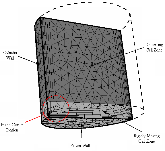
It is preferable (and even mandatory, if the mesh is a half model with a symmetry plane) to decompose the volume such that the “corner” region of the prism layers (shown in the previous figure) exists entirely within the rigidly moving zone. This allows for the largest deformations without risking degenerate elements, because the prism normals of the remeshed cells are uniformly perpendicular to the faces undergoing remeshing.
If the range of motion does not allow you to encapsulate the entire corner region of the prism layers in a rigidly moving zone, it is recommended that you encapsulate the “base” of the prism layers (shown in Figure 13.45: Volume Decomposition for the Base of the Prism Layers) and move these cells with a rigid body motion. Although this is less ideal than encapsulating the corner region, it does reduce the risk of degenerate mesh elements.
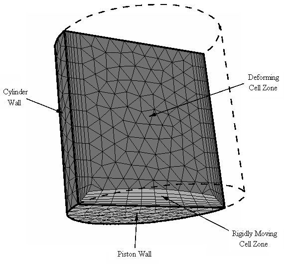
For piston-type applications that contain prism layers, a reasonable rule of thumb is that you should decompose the mesh volume if the piston motion is more than half the cylinder height. If you decide not to decompose the volume at all, you must at the very least enable the Deform Adjacent Boundary Layer with Zone option in the Meshing Options tab of the Dynamic Mesh Zone dialog box when setting up the moving face zone (see Rigid Body Motion for details). In any case, it is recommended that you always preview the mesh motion over the complete simulation time, to make sure that you will have a valid mesh at each time step.
The prism layer parameters (that is, element height, growth rate, and number of layers)
are extracted automatically from the mesh and do not generally require your input. To
prevent the prism parameters from drifting due to repeated remeshing, the prism parameters
for first height, growth rate, and number of layers can be entered manually, using the text
commands available in the
define/dynamic-mesh/controls/remeshing-parameters/prism-layer-parameters
menu.
Note the following limitations associated with face region remeshing:
You can use the face region remeshing method only in cell zones that contain triangular cells (in 2D) or tetrahedral cells, with or without prism layers (in 3D). For 3D meshes, the faces on the deforming boundaries that border the moving face must all be triangular.
The face region remeshing method is not compatible with diffusion-based smoothing or linearly elastic solid smoothing.
You cannot use the face region remeshing method in conjunction with adaption. For more information on the available adaption methods, see Hanging Node Adaption and Polyhedral Unstructured Mesh Adaption in the Theory Guide.
The 2.5D surface remeshing method only applies to extruded 3D geometries and is similar to local remeshing in two dimensions on a triangular surface mesh (not a mixed zone). Faces on a deforming boundary are marked for remeshing based on face skewness, minimum and maximum length scale; the 2.5D remeshing method also gives you the option of marking cells using sizing functions, as described in Local Remeshing Based on Sizing Function.
Figure 13.46: Close-Up of 2.5D Extruded Flow Meter Pump Geometry Before Remeshing and Laplacian Smoothing
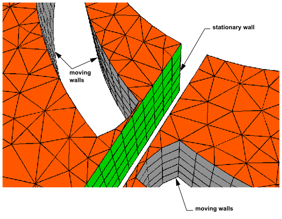
Figure 13.47: Close-Up of 2.5D Extruded Flow Meter Pump Geometry After Remeshing and Laplacian Smoothing
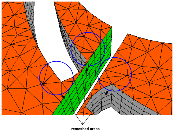
The following applies to the 2.5D surface remeshing method:
Triangular faces get remeshed based on marking.
Extruded wedges get remeshed based on the remeshing of the triangular face. Only extruded regions get remeshed, not mixed regions.
The 2.5D remeshing method does not support remeshing or moving nodes on the perimeter of the extruded zone(s).
The only smoothing method that is compatible with 2.5D remeshing is Laplacian smoothing.
Note that you cannot use the 2.5D surface remeshing method in conjunction with adaption. For more information on the available adaption methods, see Hanging Node Adaption and Polyhedral Unstructured Mesh Adaption in the Theory Guide.
The extrusion must be along a straight line normal to the deforming zone and the cross-section of the extruded/coopered mesh must be constant along the extrusion direction. For more information about the 2.5D model, see Using the 2.5D Model.
Periodics are not supported at the extruded zones.
For 3D simulations only, you can select the 2.5D model under the Remeshing tab in the Mesh Method Settings Dialog Box. This model allows for a specific subset of remeshing techniques.
The 2.5D mesh essentially is a 2D triangular mesh which is expanded, or extruded, along the normal axis of the specific dynamic zone that you are interested in modeling. The triangular surface mesh is remeshed and smoothed on one side, and the changes are then extruded to the opposite side. Rigid body motion is applied to the moving face zones, while the triangular extrusion surface is assigned to a deforming zone with remeshing and smoothing enabled. The opposite side of the triangular mesh is assigned to be a deforming zone as well, with only smoothing enabled, as in Figure 13.49: 2.5D Extruded Gear Pump Geometry.
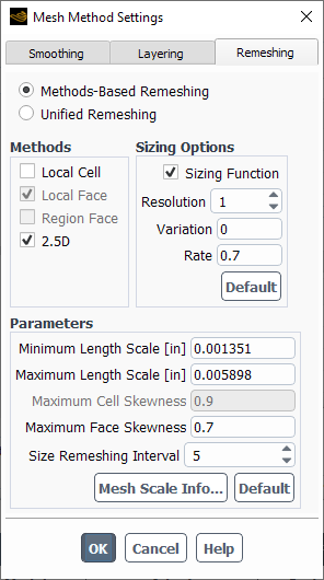
For more information on setting smoothing and remeshing parameters, see Dynamic Mesh Update Methods.
The 2.5D model only applies to mappable (that is, extrudable) mesh geometries such as pumps, as in Figure 13.49: 2.5D Extruded Gear Pump Geometry. Only the aspects of the geometry that represent the “moving parts” must be extruded in the mesh.
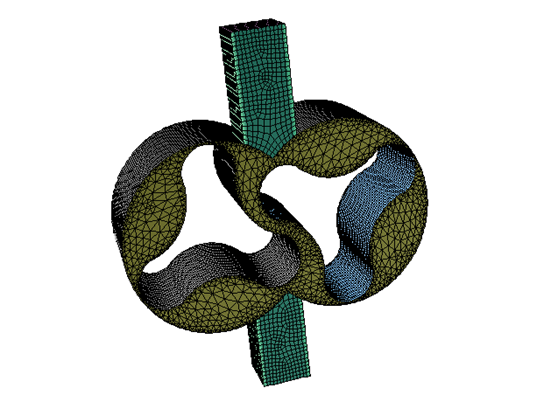
Important: You must only apply smoothing to the opposite side of the extruded mesh, since Ansys Fluent requires the geometry information for the dynamic zone. Ansys Fluent projects the nodes back to its geometry after the extrusion. Without this geometry information, the dynamic zones tends to lose its integrity.
Important: In parallel, a partition method that partitions perpendicular to the extrusion surface should be used. For example, if the normal of the extrusion surface points in the X-direction then Cartesian-Y or Cartesian-Z would be the perfect partition methods.
The 2.5D model is used in combination with a
DEFINE_GRID_MOTION UDF. (See Hooking DEFINE_GRID_MOTION UDFs in the Fluent Customization Manual for information about hooking this UDF.)
This UDF is associated with the extrusion surface that is adjacent to the cell zone, in turn applying the same deformation to the entire cell zone. This approach is particularly useful when modeling gear pumps that are predominantly extruded hexahedral meshes. For more information about this UDF, contact your support engineer.
When Unified Remeshing is selected in the Remeshing tab of the Mesh Method Settings dialog box, the mesh quality is improved using an algorithm that combines aspects of a variety of remeshing methods and by default attempts to maintain the initial mesh size distribution even as the mesh moves. Unified Remeshing simplifies the remeshing setup and can provide increased robustness compared to other methods, especially for parallel simulations.
If the default settings of the Unified Remeshing method do not yield a desirable mesh distribution for your simulation, you can attempt to improve it by clicking the button and using the Advanced Remeshing Settings dialog box that opens. The value of the Maximum Cell Skewness sets the threshold for remeshing cells based on skewness, and by default is set to 0.9 for 3D simulations and 0.7 for 2D simulations. For 3D cases, faces (and adjacent cells) on the boundaries of deforming or user-defined zone types are remeshed based on the Maximum Face Skewness.
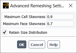
If necessary, you can disable the Retain Size Distribution option, so that algorithm does not attempt to respect the initial mesh distribution by using local size criteria, but instead marks cells for remeshing when their length scales are outside of the minimum and maximum length scale values of the cell zone in the initial mesh. Should these zonal values be unsuccessful, you can use the following text commands to specify other appropriate length scale values:
define →
dynamic-mesh → controls →
remeshing-parameters → length-min
and
define →
dynamic-mesh → controls →
remeshing-parameters → length-max
The mesh is evaluated at every time step, and the remeshing is applied only if the quality of the cells / faces has improved.
Note:
Unified remeshing is applied to triangular or tetrahedral cells, and can produce wedge cells in 3D boundary layer meshes.
You cannot use unified remeshing in conjunction with adaption. For more information on the available adaption methods, see Hanging Node Adaption and Polyhedral Unstructured Mesh Adaption in the Theory Guide.
You have the option of creating additional controls that can affect the size
distribution of the cells throughout the mesh or just the wedge cells in boundary layers by
using the
define/dynamic-mesh/controls/remeshing-parameters/sizing-controls or
define/dynamic-mesh/controls/remeshing-parameters/prism-controls/
text command menus, respectively. It is generally not necessary to create such controls, but
they may be helpful if you have strict sizing requirements or want more information when
troubleshooting size-related issues. Note that any sizing controls and/or prism controls
created in the meshing mode as part a Watertight Geometry meshing guided
workflow (as described in Using the Watertight Geometry Meshing Guided Workflows) are
automatically imported and used as part the Unified Remeshing. For
further details, see the following sections:
When the Retain Size Distribution option is enabled in the Advanced Remeshing Settings dialog box, you can use one or more sizing controls to modify the algorithm that attempts to respect the initial mesh distribution during unified remeshing. Each sizing control definition is applied to one or more boundary zones, and then affects the size of the cells throughout the mesh based on their distance from those boundary zone(s) and your settings in the definition. Any sizing controls created in the meshing mode as part a Watertight Geometry meshing guided workflow (as described in Using the Watertight Geometry Meshing Guided Workflows) are automatically imported and used; you can choose to edit and/or delete these, and/or create new controls.
Warning: Sizing controls should be used with caution by experienced users only, as they could make your simulation less robust if used incorrectly.
To create and manage sizing controls, perform the following steps:
Define a sizing controls definition using the following text command:
define→dynamic-mesh→controls→remeshing-parameters→sizing-controls→addAfter being prompted for a name, you can enter the following to complete the definition:
zonesThis specifies all of the boundary zones on which the sizing controls definition is applied.
growth-rateThis sets the growth rate of the sizing controls definition.
motionThis determines whether the evaluation of the sizing of the cells that result from the sizing control definition is updated when zones move:
autospecifies that Fluent updates the evaluation during motion; andstaticspecifies that the evaluation is not updated during motion.typeThis specifies how the sizing is affected by the selected boundary zones:
autospecifies that the default size distribution (rather than the initial size distribution in your selected boundary zones) is used, along with your specifiedmax-lengthandmin-lengthvalues;softspecifies that the maximum length scale of your selected boundary zones is used, along with your specifiedmin-lengthvalue; andmeshedspecifies that the maximum and minimum length scales of your selected boundary zones are used, in order to respect their initial size distribution. This setting is only relevant if you have more than one sizing controls definition.max-lengthThis sets a maximum length threshold that is used when the
typeis set toautoorsoft.min-lengthThis sets a minimum length threshold that is used when the
typeis set toauto.intervalThis sets the interval (in time steps) at which the evaluation of the sizing of the cells that result from the sizing control definition is updated. This setting is only relevant when
autois selected for themotionsetting. By default, theintervalis set to10time steps. This setting does not typically need to be adjusted: you could decrease it if you are using large time steps (which is not recommended), and you could increase it if it negatively impacts the calculation speed.nameYou can use this to revise the name you entered when you created the sizing controls definition.
When the definition is complete, enter
qto return to the text command menu.You can repeat the previous step if you would like additional sizing controls definitions.
You can perform the following actions as needed prior to running the calculation:
To edit an existing sizing controls definition, use the following text command:
define→dynamic-mesh→controls→remeshing-parameters→sizing-controls→editTo delete an existing sizing controls definition, use the following text command:
define→dynamic-mesh→controls→remeshing-parameters→sizing-controls→deleteTo print a list of the existing sizing controls definitions in the console, use the following text command:
define→dynamic-mesh→controls→remeshing-parameters→sizing-controls→listTo print the properties of an existing sizing controls definition in the console, use the following text command:
define→dynamic-mesh→controls→remeshing-parameters→sizing-controls→list-properties
When the Retain Size Distribution option is enabled in the Advanced Remeshing Settings dialog box, you can use one or more prism controls to modify the algorithm that attempts to respect the initial mesh distribution during unified remeshing. Each prism control definition is applied to one or more boundary zones, and then affects the height distribution and number of layers of the wedge cells in the adjacent boundary layers. Any prism controls created in the meshing mode as part a Watertight Geometry meshing guided workflow (as described in Using the Watertight Geometry Meshing Guided Workflows) are automatically imported and used; you can choose to edit and/or delete these, and/or create new controls.
Warning: Prism controls should be used with caution by experienced users only, as they could make your simulation less robust if used incorrectly.
To create and manage prism controls, perform the following steps:
Define a prism controls definition using the following text command:
define→dynamic-mesh→controls→remeshing-parameters→prism-controls→addAfter being prompted for a name, you can enter the following to complete the definition:
zonesThis specifies all of the boundary zones on which this prism controls definition is applied.
nlayersThis sets the number of layers of wedge cells in the boundary layer adjacent to the specified
zones.growth-methodThis specifies the method used to determine the increase in height of the wedge cell layers beyond the first layer. The only available option is
geometric, so that the height of each layer is the height of the previous layer multiplied by therate.rateThis sets the coefficient for the
growth-methodused to determine the increase in height of the wedge cell layers beyond the first layer.offset-typeThis allows you to select from the following types, in order to determine how the first layer of wedge cells (adjacent to the
zones) are generated during remeshing:uniformThis specifies that every new node (child) of the first layer of wedge cells is the same distance away from its parent node (that is, the corresponding node on the boundary zone, from which the direction vector is pointing). This distance is defined by the
first-height. Theuniformtype is selected by default.aspect-ratioThis specifies that the first layer of wedge cells that are extruded from the
zonesare defined using an aspect ratio, that is, the ratio of the local wedge base length (as averaged at the nodes) to the local wedge layer height. This aspect ratio is defined by thefirst-aspect-ratio. Note that for a uniform mesh, the heights of the cells in the first layer will be roughly the same, while for a varying mesh, these heights will vary.smooth-transitionThis specifies that the last layer of wedge cells that are extruded from the
zonesare defined using a transition rate, that is, the ratio of the local wedge cell height (as averaged at the nodes) to the height of the local tetrahedral cell that will be generated adjacent to the last layer. This transition rate / ratio is defined by thetransition-rate. This offset type allows you to easily provide a smooth transition for the cell volumes from the wedge cell layers to the cells deeper within the mesh. After the height of the last wedge cell layer is calculated, the height of the first layer is automatically computed according to your specified growthrateandnlayers. Note that for a uniform mesh, the heights of the cells in the first layer will be roughly the same, while for a varying mesh, these heights will vary.
These offset types are similar to the offset method types available when adding boundary layers in a Watertight Geometry guided workflow in the meshing mode (as described in Adding Boundary Layers). For further details about how the
uniformandaspect-ratiotypes affect the placement of the nodes during remeshing, see Offset Distances.first-heightThis sets the height of the first layer of wedge cells in the boundary layer adjacent to the specified
zones. It is used whenuniformis selected for theoffset-type(which is the default).first-aspect-ratioThis sets the aspect ratio for the individual wedge cells in the first layer of cells adjacent to the specified
zones. It is defined as the ratio of the local wedge base length (as averaged at the nodes) to the local wedge layer height. It is used whenaspect-ratiois selected for theoffset-type.transition-rateThis sets the ratio of the local wedge cell height (as averaged at the nodes) in the last wedge cell layer to the height of the local tetrahedral cell that will be generated adjacent to the last layer (deeper within the mesh). It is used when
smooth-transitionis selected for theoffset-type.nameYou can use this to revise the name you entered when you created the prism controls definition.
When the definition is complete, enter
qto return to the text command menu.You can repeat the previous step if you would like additional prism controls definitions.
You can perform the following actions as needed prior to running the calculation:
To edit an existing prism controls definition, use the following text command:
define→dynamic-mesh→controls→remeshing-parameters→prism-controls→editTo delete an existing prism controls definition, use the following text command:
define→dynamic-mesh→controls→remeshing-parameters→prism-controls→deleteTo print a list of the existing prism controls definitions in the console, use the following text command:
define→dynamic-mesh→controls→remeshing-parameters→prism-controls→listTo print the properties of an existing prism controls definition in the console, use the following text command:
define→dynamic-mesh→controls→remeshing-parameters→prism-controls→list-properties
The volume mesh is updated automatically based on the methods described in Dynamic Mesh Update Methods. Ansys Fluent decides which method to use for a particular zone based on which model is enabled and the shape of the cells in the zone. For example, if the boundaries of a tetrahedral cell zone are moving, the mesh smoothing and local remeshing methods will be used to update the volume mesh in this zone. If the zone consists of prismatic (hexahedral and/or wedge) cells, then the dynamic layer method will be used to determine where and when to insert and remove cell layers. On extruded prism zones, the 2.5D surface meshing method will be used.
Depending on which model is enabled, Ansys Fluent automatically determines which method to use by visiting the adjacent cell zones and setting appropriate flags for the volume mesh update methods to be used. If you specify the motion for a cell zone, Ansys Fluent will visit all of the neighboring cell zones and set the flags appropriately. If you specify the motion of a boundary zone, Ansys Fluent will analyze only the adjacent cell zones. If a cell zone does not have any moving boundaries, then no volume mesh update method will be applied to the zone.
Important: Note that as a result of the remeshing procedures, updated meshes may be slightly different when dynamic meshes are used in parallel Ansys Fluent, and therefore very small differences may arise in the solutions.
Important: Note that if your dynamic mesh model consists of numerous shell conduction zones, the mesh update may be very time consuming because all shells are deleted and recreated during the mesh update.
The second order in time transient formulation can be used with remeshing, layering, and smoothing cases. In such cases, second order in time accuracy is preserved during layering events and/or mesh smoothing. However, during remeshing events, the time advancement accuracy reverts to first order. Therefore, it is recommended that you only use second order in time for cases with very low remeshing frequency, that is, for cases where remeshing occurs every several time steps or more. If remeshing occurs every time step, the method reduces to a first order formulation. For cases that need very frequent remeshing, it is recommended that you retain the first order in time formulation. For details, see Dynamic Mesh Theory in the Fluent Theory Guide.
The switch to first order happens automatically when the solver detects a topology change as a result of remeshing within a time step. You will not see a change in the user interface, however you can monitor the switch between first and second order in time by using the following text command to enable the verbosity with dynamic meshes:
define →
dynamic-mesh →
transient-settings → verbosity
A message showing the active time formulation will print to the console when verbosity is
set to 1.
Note: For cases with second order in time with dynamic mesh enabled, any mesh swapping and manual mesh manipulation will trigger a switch to first order in time.
The remeshing and/or smoothing of boundary zones may result in the chamfering of corners where cell faces meet. However, there may be some corners (identified by a particular angular range) that are important for your flow, and that you do not want chamfered. For 3D cases, you can specify that Ansys Fluent detects such corners (or "features") and preserves them. Such features may be at the juncture of different boundary zones, or they may be on a single non-planar boundary zone.
In the Geometry Definition tab of the Dynamic Mesh Zones Dialog Box for any Definition type, you can indicate whether you want to preserve features by enabling Feature Detection under Feature Options and specifying a threshold value for the Feature Angle. A value of 180 degrees (the default) for the Feature Angle means that none of the corners must be preserved, whereas a value of 0 means that all of the corners must be preserved.
To illustrate the setting of the Feature Angle, see Figure 13.51: Cross Section of a 3D Corner. If you set the Feature Angle to 40 degrees, this corner would be guaranteed to be preserved. If you set it to 50 degrees, this corner could be chamfered.
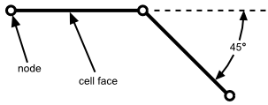
The following items are applicable for use with feature detection:
Feature remeshing is only possible with face region remeshing.
Features are preserved by local face remeshing, that is, there is no local face remeshing across features.
Smoothing methods preserve features, that is, nodes at feature edges are not allowed to be smoothed.
You can enable the In-Cylinder option in the Dynamic Mesh Task Page (Figure 13.13: The Dynamic Mesh Task Page) for transient problems. Then click the button in the Options group box to open the Options Dialog Box. Click the In-Cylinder tab and specify the Crank Shaft Speed, the Starting Crank Angle, and the Crank Period, which are used to convert between flow time and crank angle. You must also specify the time step size to use for advancing the solution in terms of crank angle in Crank Angle Step Size. By default, Ansys Fluent assumes a Crank Angle Step Size of 0.5 degrees.
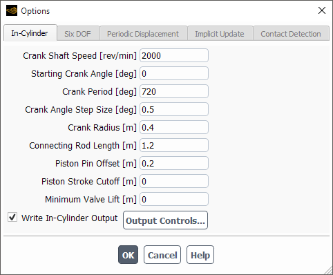
Ansys Fluent provides a built-in function that can define the location of the piston as a function of crank angle. This function is named **piston-full**, and is selected from the Motion UDF/Profile drop-down list in the Dynamic Mesh Zones dialog box as part of rigid body motion (see Rigid Body Motion for details). If you plan to specify the piston motion using this function, you must specify the Crank Radius (that is, the distance between the crank center and the center of the crank pin) and the Connecting Rod Length. You also have the option of entering a value for the Piston Pin Offset for cases when the piston pin is offset perpendicularly from the plane defined by the crank shaft axis and the direction of motion of the piston. The sign of this offset can be positive or negative, and is determined based on the geometry and the direction of rotation of the crank shaft (as shown in Figure 13.53: Determining the Sign of the Piston Pin Offset).
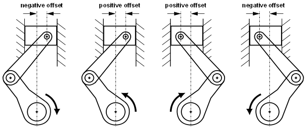
When the **piston-full** function is used, the piston location is calculated according to the following equation:
 | (13–25) |
where  is the piston location,
  the crank radius,
  is the connecting rod length,
  is
the piston pin offset, and
is
the piston pin offset, and  is the current crank angle.
The piston location  is always 0 at top-dead-center
(TDC), that is, when the crank pin is perfectly aligned between the
piston pin and the center of rotation of the crank shaft. TDC occurs
when the crank angle is 0° when there is no piston pin offset, and prior to the crank angle
reaching 0° when
there is a positive piston pin offset. The piston location is a positive
value at bottom-dead-center (BDC), that is, when the crank shaft is
perfectly aligned between the piston pin and the crank pin. The value
of
is always 0 at top-dead-center
(TDC), that is, when the crank pin is perfectly aligned between the
piston pin and the center of rotation of the crank shaft. TDC occurs
when the crank angle is 0° when there is no piston pin offset, and prior to the crank angle
reaching 0° when
there is a positive piston pin offset. The piston location is a positive
value at bottom-dead-center (BDC), that is, when the crank shaft is
perfectly aligned between the piston pin and the crank pin. The value
of  at BDC is equal to
  when
there is no piston pin offset, and greater than
when
there is no piston pin offset, and greater than  when there
is a nonzero piston pin offset (positive or negative).
when there
is a nonzero piston pin offset (positive or negative).
The current crank angle  is calculated from
 | (13–26) |
where  is the Starting Crank Angle and
  is the Crank Shaft Speed.
The Piston Stroke Cutoff and Minimum Valve Lift values are used to control the actual values of the valve lift and piston stroke such that
 | (13–27) |
where  is the valve lift
computed from the appropriate valve profiles,
is the valve lift
computed from the appropriate valve profiles,  is the Minimum Valve
Lift,
is the Minimum Valve
Lift,  is the stroke calculated
from Equation 13–25, and
is the stroke calculated
from Equation 13–25, and  is the Piston Stroke
Cutoff. (See Defining Motion/Geometry Attributes of Mesh Zones on how the Piston Stroke Cutoff is used to
control the onset of layering in the cylinder chamber.)
is the Piston Stroke
Cutoff. (See Defining Motion/Geometry Attributes of Mesh Zones on how the Piston Stroke Cutoff is used to
control the onset of layering in the cylinder chamber.)
Enable the Write In-Cylinder Output option then click the button if you want to specify specific output parameters. The In-Cylinder Output Controls Dialog Box will open, where you can specify various quantities needed for the calculation of swirl and tumble along with the frequency of writing the output to the chosen file. Swirl is used to describe circulation about the cylinder axis. Tumble flow circulates around an axis perpendicular to the cylinder axis, orthogonal to swirl flow.
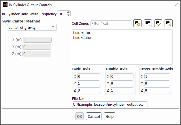
The following list describes the In-Cylinder Output Controls Dialog Box.
- In-Cylinder Data Write Frequency
is an integer entry specifying the interval in number of time-steps. Make sure that a value other than 0 is used for the frequency, in order to allow you to complete your setup.
- Swirl Center Method
is a drop-down list that allows you to select the method to calculate the swirl center. The list contains center of gravity and fixed, with center of gravity being the default value.
- center of gravity
option calculates the swirl center inside the code and is used as the center of gravity of the chosen cell zones.
- fixed
option enables you to specify a swirl center in the entries below the drop-down list.
In addition to these two options, you can chose to use your own compiled UDF to calculate the swirl center.
For details on using a dynamic mesh UDF, see the Fluent Customization Manual for information on user-defined functions.
- Cell Zones
is a list that displays the names of all existing cell zones in the case files. You can select only the zones relevant for the swirl and tumble calculations.
- Swirl Axis
specifies the swirl axis with three entries for the directional components. By default, X, Y, Z = 0, 1, 0.
- Tumble Axis
specifies the directional components of Tumble Axis in X, Y, Z directions. By default, X, Y, Z = 0, 0, 1. This applies only in 3D.
- Cross Tumble Axis
specifies the directional components of Cross Tumble Axis in X, Y, Z directions. By default, X, Y, Z = 1, 0, 0. This applies only in 3D.
- File Name
specifies the name of the In-Cylinder output file. By default, the file name contains the name of the case file appended with a
.txtextension.
The In-Cylinder specific output controls can also be controlled using the TUI as follows:
Go to define/dynamic-mesh/controls/in-cylinder-output? Enable in-cylinder output?[no]yesOutput Write Frequency[0]10Cell zone name/id(1)[()]2Cell zone name/id(1)[()] File Name[‘‘/nfs/devvault/data9/ic-sp-output.txt’’] Swirl Center Method: (fixed cg user-defined)Option[cg] Swirl Axis x[0] Swirl Axis y[1] Swirl Axis z[0] Tumble Axis x[0] Tumble Axis y[0] Tumble Axis z[1] Cross Tumble Axis x[1] Cross Tumble Axis y[0] Cross Tumble Axis z[0]
If you select fixed as the choice at Swirl Center Method then you will be prompted to enter the swirl center as follows:
 Swirl Center(x) (mm) [0]
 Swirl Center(y) (mm) [0]
 Swirl Center(z) (mm) [0]
If a swirl center method UDF has been compiled already and loaded into UDF then you can choose user-defined as the swirl center method option, in such a case the following is the sequence of prompts.
Swirl Center UDF[] swirl_udf::libudf
If the name of the UDF library is libudf then you can omit this and enter in the swirl center UDF[]swirl_udf, otherwise the name of the UDF followed
by the UDF library name with symbol:: in between, should be entered.
By filling up the various entries that are needed in the In-Cylinder Output Controls Dialog Box and pressing the button, the swirl and tumble calculations will be written at the chosen frequency to the chosen file while doing the solution run. Details of the quantities written to the file are as follows:
|
CA = Crank Angle |
|
m = Mass of the entire fluid contained in the selected cell zones |
|
L = Angular momentum vector of fluid mass contained in selected cell zones with respect to the swirl center |
|
|
|
|
|
|
|
|
|
I |
|
I |
|
I |
|
|


Altogether, the previous quantities are combined to yield eight columns of data in the output file, as shown in the figure that follows:
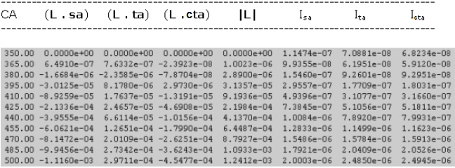
This section describes the problem setup procedure for an in-cylinder dynamic mesh simulation.
Consider the 2D in-cylinder example shown in Figure 13.56: A 2D In-Cylinder Geometry for a typical pent-roof engine.
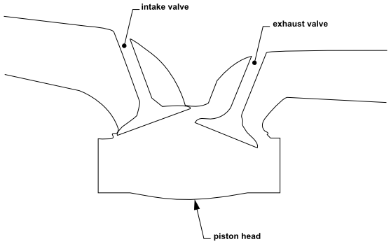
In setting up the dynamic mesh model for an in-cylinder problem, you must consider the following issues:
how to provide the proper mesh topology for the volume mesh update methods (smoothing, dynamic layering, and local or zonal remeshing)
how to define the motion attributes and geometry for the valve and piston surfaces
how to address the opening and closing of the intake and exhaust valves
how to specify the sequence of events that controls the in-cylinder simulation
Ansys Fluent requires that you provide an initial volume mesh with the appropriate mesh topology such that the various mesh update methods described in Dynamic Mesh Update Methods can be used to automatically update the dynamic mesh. However, Ansys Fluent does not require you to set up all in-cylinder problems using the same mesh topology. When you generate the mesh for your in-cylinder problem, you must consider the various mesh regions that you can identify as moving, deforming, or stationary, and generate these mesh regions with the appropriate cell shape.
The mesh topology for the example problem in Figure 13.56: A 2D In-Cylinder Geometry is shown in Figure 13.57: Mesh Topology Showing the Various Mesh Regions, and the corresponding volume mesh is shown in Figure 13.58: Mesh Associated With the Chosen Topology.
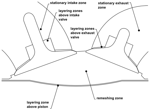
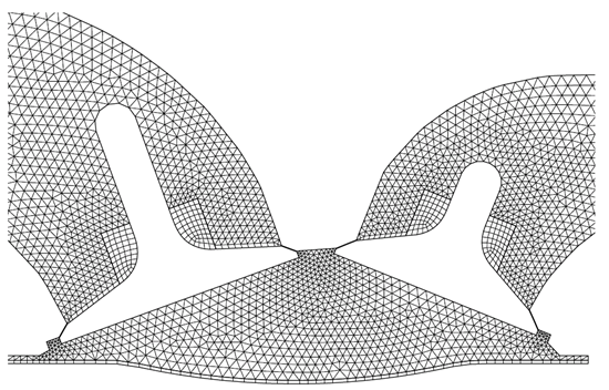
Because of the rectilinear motion of the moving surfaces, you can use dynamic layering zones to represent the mesh regions swept out by the moving surfaces. These regions are the regions above the top surfaces of the intake and exhaust valves and above the piston head surface, and must be meshed with prismatic cells that are quadrilateral in 2D or polyhedral, hexahedral, or wedge cells in 3D (as required by the dynamic layering method).
For the chamber region, you must define a remeshing zone (triangular cells) to accommodate the various positions of the valves in the course of the simulation. In this region, the motion of the boundaries (valves and piston surfaces) is propagated to the interior nodes through smoothing. If the cell quality violates any of the remeshing criteria that you have specified, Ansys Fluent will automatically agglomerate these cells and remesh them. Furthermore, Ansys Fluent will also remesh the deforming faces (based on the minimum and maximum length scale that you have specified) on the cylinder walls as well as those on the sliding interfaces used to connect the chamber cell zone to the layering zones above the valve surfaces.
For the intake and exhaust port regions, you can use either triangular or quadrilateral cell zones because these zones are not moving or deforming. Ansys Fluent will automatically mark these regions as stationary zones and will not apply any mesh motion method on these cell zones.
The dynamic layering regions above the piston and valves are conformal with the adjacent cell zone in the chamber and ports, respectively, so you do not have to use sliding interfaces to connect these cell zones together. However, you must use sliding interfaces to connect the dynamic layering regions above the valves and the remeshing region in the chamber. This is shown in Figure 13.59: The Use of Sliding Interfaces to Connect the Exhaust Valve Layering Zone to the Remeshing Zone with the exhaust valve almost at full extension. Notice that cells on the chamber side of the interface zone are remeshed (that is, split or merged) as the interface zone opens and closes because of the motion of the exhaust valve.
Figure 13.59: The Use of Sliding Interfaces to Connect the Exhaust Valve Layering Zone to the Remeshing Zone
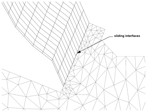
As the piston moves down from the TDC to the BDC position, you
must expand the remeshing region such that it can accommodate the
valves when they are fully extended. To accomplish this, you must
specify the dynamic layering zone adjacent to the piston surface to
move with the piston until some specified distance from the TDC position.
Beyond this cutoff distance, the motion of the layering zone is stopped
and the piston wall is allowed to continue to the BDC position. Because
there is relative motion between the piston head surface and the now
non-moving dynamic layering zone, cell layers will be added when the
ideal layer height criteria is violated. Figure 13.60: Mesh Sequence 1 to Figure 13.65: Mesh Sequence 6 show the sequence of meshes
before and after the onset of cell layering when the motion in the
layering zone above the piston surface is stopped (shown with  = 5°).
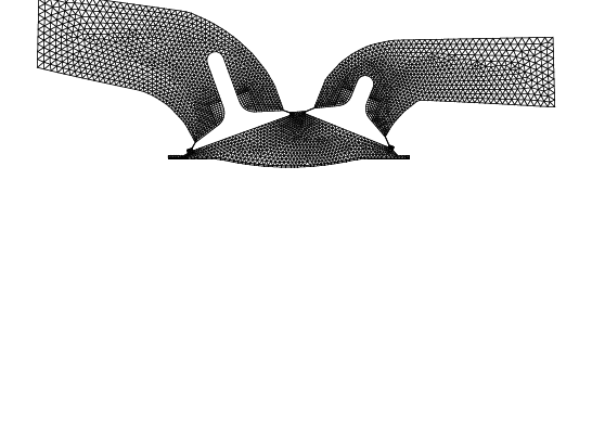
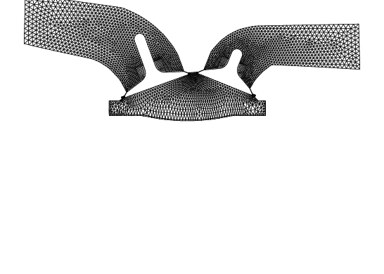
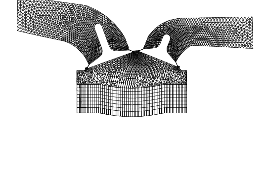
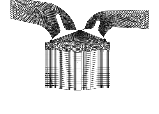
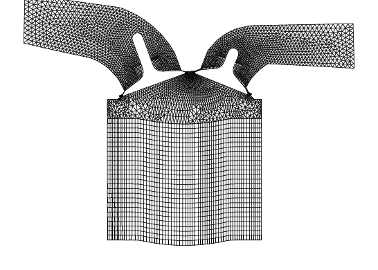
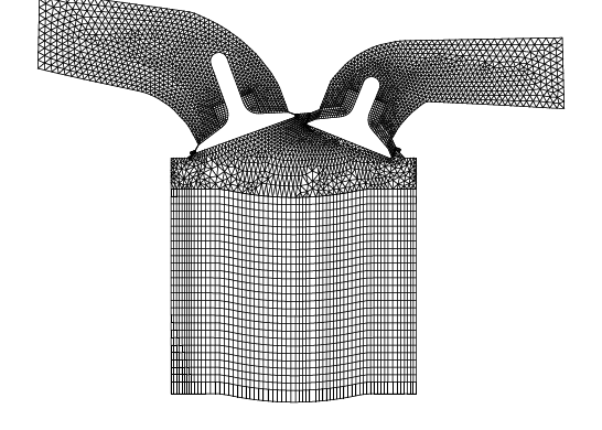
Ansys Fluent provides built-in functions to handle the full
piston motion and the limited piston motion for the dynamic layering
zone above the piston surface. When you define the motion attribute
of the dynamic layering zone above the piston surface, you must use
the limited piston motion function (**piston-limit** in the Motion UDF/Profile field in the Dynamic Mesh Zones Dialog Box). Note that you must define
the parameters used by these functions before you can use them. In
the current example, the crank radius is 40 mm and the connecting
rod length is 140 mm. The piston stroke cutoff is assumed to
happen at 25 mm from TDC position. The lift as a function of
crank angle between  and
and  is shown in Figure 13.66: Piston Position (m) as a Function of Crank Angle (deg) for both limited and full piston
motion.
is shown in Figure 13.66: Piston Position (m) as a Function of Crank Angle (deg) for both limited and full piston
motion.
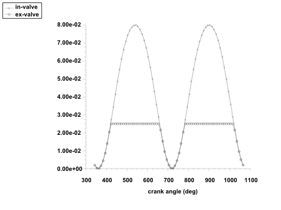
To define the motion of the valves, you must use profiles that describe the variation of valve lift with crank angle. Ansys Fluent expects certain profile fields to be used to define the lift and the crank angle. For example, consider the following simplified profile definition:
 ((ex-valve 5 point)
 (angle 0  180 270 360  720)
 (lift 0.05 0.05 1.8 0.05 0.05))

 ((in-valve 5 point)
 (angle 0  355  440 540 720)
 (lift 0.05 0.05 2.0 0.05 0.05))
Ansys Fluent expects the angle and lift fields to define the crank angle and lift variations,
respectively. The angle must be specified in degrees and the lift
values must be in meters. The actual valve lift profiles that you
will use for the current example are shown in Figure 13.67: Intake and Exhaust Valve Lift (m) as a Function of Crank Angle
(deg). Notice that there is an overlapped
period where both the intake and exhaust valves are open.
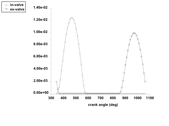
The valve lift profiles and the built-in functions will describe how each surface moves as a function of crank angle with respect to some reference point. For example, the valve lift is zero when the valve is fully closed and the valve lift is maximum when it is fully open. In order to move the surfaces, Ansys Fluent requires that you specify the direction of motion for each surface. Ansys Fluent will then update the “center of gravity” of each surface such that
 | (13–28) |
where  is some reference position,
  is the unit
vector in the direction of motion, and
is the unit
vector in the direction of motion, and  is either the valve or the piston
distance with respect to the reference position
is either the valve or the piston
distance with respect to the reference position  . Note that the unit vector
of the direction of motion is specified to point in the negative direction.
For example, the correct intake valve axis for this example is
. Note that the unit vector
of the direction of motion is specified to point in the negative direction.
For example, the correct intake valve axis for this example is  , as shown
in Figure 13.68: Definition of Valve Zone Attributes (Intake Valve).
, as shown
in Figure 13.68: Definition of Valve Zone Attributes (Intake Valve).
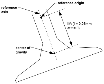
Ansys Fluent assumes that once you have set up the mesh topology, the mesh topology is unchanged throughout the entire simulation. Therefore, Ansys Fluent does not allow you to completely close the valves such that the cells between the valve and the valve seat become degenerate (flat cells) when these surfaces come in contact (removing these flat cells would require the creation of new boundary face zones). To prevent the collapse, you must define a minimum valve lift and Ansys Fluent will automatically stop the motion of the valve when the valve lift is smaller than the minimum valve lift value. The minimum valve lift value can be specified in the In-Cylinder tab of the Options Dialog Box. For the current example, a minimum valve lift value of 0.1 mm is assumed.
When the valve position is smaller than the minimum valve lift value, it is normal practice to assume that the valve is closed. The actual closing of the valves is accomplished by deleting the sliding interfaces that connect the chamber cell zone to the dynamic layering zones on the valves. The interface zones are then converted to walls to close off the “gaps” between the valves and the valve seats.
The valve opening is achieved by the reverse process. When the valve lift has reached beyond the minimum valve lift value, the valve is assumed to be open and you can redefine the sliding interfaces such that the chamber zone is now connected to the dynamic layering zones above the valves.
Ansys Fluent’s six degrees of freedom (six DOF) solver computes external forces and moments (such as aerodynamic and gravitational forces and moments) on objects that undergo rigid body motion. These forces are computed by numerical integration of pressure and shear stress over the object’s surfaces. Additional load forces can be added, such as injector forces, thrust (propulsive) forces, and moments produced by a coil spring. This technique, along with the Ansys Fluent solver and the use of dynamic meshes, can be readily applied to many useful applications, such as store separation [140], [151]. Note that the objects may be composed of multiple zones.
To use the six degrees of freedom solver for your transient dynamic mesh simulation, perform the following steps:
Enable the Six DOF option in the Options group box of the Dynamic Mesh Task Page (Figure 13.13: The Dynamic Mesh Task Page) and click the button. The Options dialog box will open, where you can click the Six DOF tab (Figure 13.69: The Six DOF Tab of the Options Dialog Box).
This tab allows you to perform the following actions:
You can create and manage sets of six DOF properties for rigid body motion by using the list and buttons under Six DOF Properties; otherwise, you will have to create one or more user-defined functions. See Setting Rigid Body Motion Attributes for the Six DOF Solver for details.
You can specify the gravitational acceleration for the x, y, and z directions either in this dialog box, or in the Operating Conditions dialog box.
You can keep track of an object’s motion history by enabling the Write Motion History option and entering a File Name. A single motion history file will be generated for each moving object, which can be used to display zone motion for postprocessing your results. Note that the file name you specify will be appended with the name of the set of six DOF properties / UDF, as well as the extension
.6dof; you can change the extension by specifying your own as part of the File Name.
If the mesh motion of your six DOF simulation depends on the fluid flow, it is beneficial to enable implicit mesh updating (as described in Implicit Update Settings). If the implicit mesh update is not sufficient to stabilize the solver due to the fluid motion, solution stabilization may be necessary. The solution stabilization settings are set in the Solver Options tab of the Dynamic Mesh Zones dialog box for boundary zones (Solution Stabilization for Dynamic Mesh Boundary Zones).
Define the rigid-body zone(s) that make up each moving object by using the Dynamic Mesh Zones Dialog Box, as described in Rigid Body Motion.
Setup → Dynamic
Mesh → Create/Edit...
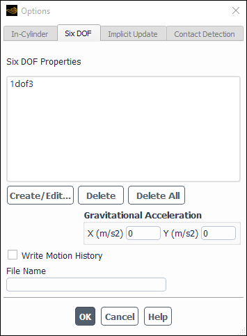
As part of the six DOF solver settings, you must provide either a set of properties or a user-defined function (UDF) for each moving object, in order to define its overall mass, rotational inertia, constraints, loading from sources other than aerodynamics and gravity, and so on. Each object needs exactly one set of properties / UDF, regardless of how many zones make up the object. Note that if you have multiple identical objects, you can create an initial set of properties / UDF, and then make copies with unique names.
If the motion of the object is complex or if only half of the object is modeled using a
symmetry zone, then you will need to use a UDF (see
DEFINE_SDOF_PROPERTIES
in the Fluent Customization Manual for the details);
otherwise, it is easier to use a set of properties. Such sets are created using the
Six DOF Properties dialog box, which is opened by clicking the
button in the Six DOF tab of the
Options Dialog Box.
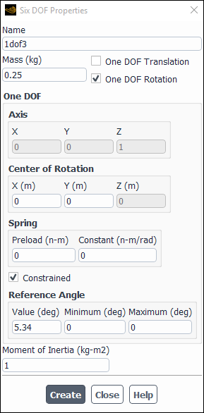
In the Six DOF Properties dialog box, you will need to provide a Name for the set of properties, define the other fields in the dialog box, and click .
For six DOF motion, the only other fields that must be defined are the Mass and the Inertia Tensor components. Note that the inertia tensor components are defined relative to the Center of Gravity and Rigid Body Orientation settings defined in the Dynamic Mesh Zones Dialog Box; the latter settings allow you to use a coordinate system that is local (rather than global), if that is more convenient.
If you want to specify that the dynamic object be limited to one DOF motion (that is, either a simple translation or a simple rotation), enable the One DOF Translation or One DOF Rotation option and define the settings in the One DOF group box. The following figure shows an example of a one DOF translation:
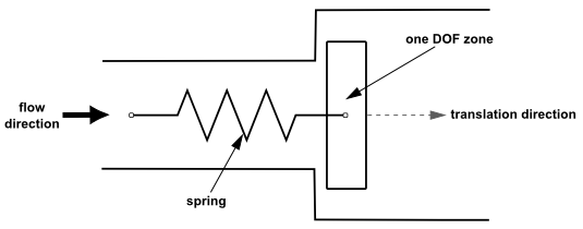
Note the following about one DOF motion settings:
For rotation, you will define the Mass of the dynamic object, in case the Center of Rotation is different than the Center of Gravity defined in the Dynamic Mesh Zones Dialog Box (which may be the case in a swinging pendulum, for example), so that Fluent can calculate the moment due to gravity.
For rotation, you will also define the Moment of Inertia, as calculated around the Center of Rotation and Axis. Fluent calculates the moment of fluid forces about the Center of Rotation. Note that this definition of the Moment of Inertia is different from a six DOF case that does not use One DOF Rotation, where you would calculate the Inertia Tensor relative to the Center of Gravity and Rigid Body Orientation settings defined in the Dynamic Mesh Zones Dialog Box, as noted previously.
For 2D cases with rotation, the axis will be either the positive or negative z direction, depending on the sign of the value you enter for Z in the Axis group box.
You have the option of defining a Hooke's law Spring that exerts forces / torques on the dynamic object. It is a compression / extension spring for translations, and it is a torsion spring for rotations.
For example: for a translation, the specified Constant will be multiplied by the distance of the dynamic object from its initial location. This force will be combined with a Preload value that is constantly applied to the dynamic object, in order to produce the net spring loading. Note that the Preload can be a positive or negative value, and is defined relative to the Direction.
You can limit the range of motion of the dynamic object by enabling the Constrained option and defining the settings in the Reference Point group box (for translation) or the Reference Angle group box (for rotation).
For example: for a translation, you could enter
2inches for the Location, in order to assign a coordinate value to a point located on the dynamic object in its initial position. Then you would define the range of motion allowed relative to that coordinate: you would enter1.2and2inches for the Minimum and Maximum, respectively, if you wanted the object to only be allowed to move .8 inches in the direction opposite to the Direction vector. The value of the Location is arbitrary, and allows you to define the range using values that are most convenient for your problem.The initial position / orientation of the object (which is used to calculate the spring loading and/or range of motion) is established when you create the dynamic zone(s) using the Dynamic Mesh Zones Dialog Box.
For transient problems, you can enable implicit mesh updating when you want to have the dynamic mesh updated during a time step (as opposed to just at the beginning of a time step). This capability is beneficial only for applications in which the mesh motion depends on the flow field (for example, cases that use the six DOF solver or involve fluid-structure interaction). For such applications, having the mesh motion updated within the time step based on the converging flow solution results in a stronger coupling between the flow solution and the mesh motion, and leads to a more robust solver run. Implicit mesh updating allows you to run simulations that otherwise could not be solved or would require an unreasonably small time step size.
Note that implicit mesh updating cannot be used with the following:
the density-based solver when Explicit is selected from the Transient Formulation drop-down menu in the Solution Methods task page
steady-state solutions
in-cylinder applications
To enable implicit mesh updating, perform the following steps:
Enable Implicit Update in the Options group box of the Dynamic Mesh Task Page (Figure 13.13: The Dynamic Mesh Task Page).
Click the button to open the Options Dialog Box.
Click the Implicit Update tab and enter values for the settings.
Enter a value for Update Interval, in order to specify the frequency in iterations at which the mesh will be updated within a time step.
Enter a value (within the range of 0 to 1) for Motion Relaxation, in order to define the relaxation of the motion (that is, displacement of the nodes) during the mesh update. The relaxation of the displacements is defined by the following equation:

(13–29)
where
 is the node position at iteration
  (within a time step),
  is the computed node
position (based on the flow field), and
is the computed node
position (based on the flow field), and  is the motion relaxation.
Note: The nodal positions returned from the UDF / profile will not be relaxed according to Equation 13–29 if you select User-Defined from the Type list when setting up your dynamic mesh zones in the Dynamic Mesh Zones Dialog Box.
Enter a value for Residual Criteria, in order to set the relative residual threshold that is used to check the motion convergence. The residual criteria is applied to a relative residual. Ansys Fluent scales the difference between the motion in iteration
 and iteration
  by the motion computed at the
beginning of the time step. If this relative motion difference is
smaller than the residual criteria, the mesh motion is considered
converged.
by the motion computed at the
beginning of the time step. If this relative motion difference is
smaller than the residual criteria, the mesh motion is considered
converged.
If you are using a UDF to compute the motion, make sure that the UDF uses the current flow field during each call to compute the motion (that is, no previously stored information should be used). This is necessary, as the UDF will be called each time the mesh is updated — which can be several times within a time step, depending on what you entered for the Update Interval.
After you run the simulation, make sure that the motion (and consequently, the solution) is properly converged. If the motion requires more iterations to converge than the flow field, a warning will be displayed in the console during the iteration process. Note that the maximum number of iterations per time step (defined in the Run Calculation task page) is respected by the mesh motion convergence check.
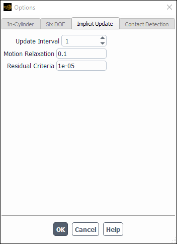
Contact detection is used to detect if the computed mesh motion will result in contact of a moving surface with other surrounding surfaces. If there is contact within a specified tolerance, then the mesh motion of the moving zone can be constrained using nodal contact information within user-defined functions (See Example 2 under DEFINE_CONTACT in the Fluent Customization Manual) and/or the flow can be controlled in the contact region.
To enable contact detection in your dynamic mesh simulation, select the Contact Detection check box in the Options group of the Dynamic Mesh task page. Click the button to open the Options dialog box and select the Contact Detection tab (see Figure 13.73: The Contact Detection Tab of the Options Dialog Box).
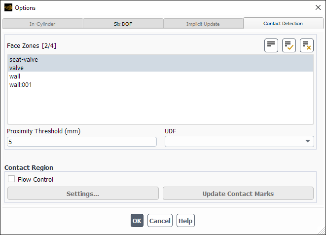
You can select the face zones that will be involved in the contact detection process from the Face Zones list. While all eligible face zones in the Face Zones list are selected by default, you can choose to exclude certain zones for efficiency. Only walls and dynamic zones of type Rigid Body or User-Defined can be selected for contact detection.
From the UDF drop-down list, you can specify a user-defined function
that will be invoked when contact has been detected. For more information about contact UDFs,
see DEFINE_CONTACT in the Fluent Customization Manual.
You must specify a Proximity Threshold value in order to enable the contact detection process. When the distance between face zones falls below this threshold value, the UDF specified in the UDF drop-down list is invoked.
You can also apply flow control in the contact region. Flow control is applied to the cells that lie within the Proximity Threshold distance of the specified face zones. There are two methods available for flow control: one based on contact zones (Flow Control Using Contact Zones), and another based on contact marks (Flow Control Using Contact Marks). To use one of these methods, enable the Flow Control option in the Contact Region group box and click the button to open the Flow Control Settings dialog box, where you can complete the setup (as described in the following sections).
Note: When simulating the complete blockage of flow between moving surfaces, it is recommended that you use the gap model rather than the Flow Control option (and the two are not compatible with each other). For details, see Controlling Flow in Narrow Gaps for Valves and Pumps.
You can select Contact Zones from the Method list in the Flow Control Settings dialog box. The Contact Zones method for controlling flow allows you to modify the flow in the contact region by creating a separate cell zone containing the marked cells. The flow in this cell zone may be controlled using the available cell zone conditions. By default, the zone is defined to have porous resistance. This method is fully compatible with all solver options.
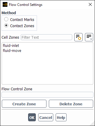
To complete the setup, you must create one or more flow control zones. Select a fluid cell zone from the Cell Zones list, specify a new name in the Flow Control Zone text box, and click the button. A new cell zone will be created that is based on the selection from the Cell Zones list, only with the Porous Zone option enabled. The Fluids dialog box will open for this new zone, allowing you to revise physical properties (for example, inertial and/or viscous porous resistance) so that it better represents the restricted flow. During the simulation, after cells in the contact region have been separated into new zones, the physical properties specified in the respective flow control zone are copied to the newly separated cell zone.
You can select Contact Marks from the Method list in the Flow Control Settings dialog box. The Contact Marks method applies a zero mass flux numerical boundary condition on the boundary of the marked contact region that blocks the flow.
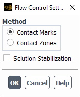
When the Contact Marks method is selected, you have the option of enabling Solution Stabilization to improve the stability of the simulation. Solution Stabilization applies solution control to stabilize the solution in the vicinity of the contact region during contact engagement, evolution, and disengagement. Solution Stabilization involves additional iterations within the time step, during which solution convergence checks are suspended.
Note that the following limitations apply when using the Contact Marks method:
It is limited to the pressure-based solver.
The use of the Green-Gauss Node Based gradient method and/or the QUICK discretization scheme is not supported.
The Non-Iterative Time Advancement (NITA) scheme is not supported.
Boundary zones of type outflow are not recommended.
For transient flows with moving face zones, the marked contact region is not fixed and could change during every time step when there is mesh motion. With the Contact Zones method, this involves deletion and recreation of the cell zone used to apply flow control; this is a computationally expensive operation. Furthermore, while the porous sources are effective in providing resistance to flow, they do not achieve complete flow blockage (which may desirable, for example, in the case of modeling the closing of a valve). Consequently, the Contact Zones method may be the recommended method for flow control only under the following conditions: complete flow blocking is not required; the flexibility of cell zone conditions to modify the flow is sufficient; and the contact region is not undergoing rapid changes.
The Contact Marks method applies a numerical zero mass flux boundary condition at the boundary faces of the region marked for contact, such that the cells in the contact region no longer participate in the solution. There are a few key advantages of this method that are important to note:
Marking is computationally more efficient than zone separation.
The flow is completely blocked at the contact region boundary and there is no flow leakage. This is a realistic flow condition for valves in the closed position.
It can reduce computational cost in narrow gaps by reducing the need for a high cell count to resolve high solution gradients in the flow between walls in close proximity (for example, a valve opening and closing).
It can avoid the difficulties of meshing and/or remeshing in narrow passages, especially with moving deforming meshes.
While there are clear advantages, there are some important considerations when using the Contact Marks method. The imposition of the zero mass flux condition on arbitrary interior boundary faces can introduce large gradients in the flow in the vicinity of the contact region boundary. Here, Solution Stabilization is recommended for cases where the engagement, evolution, and disengagement of contact can be rather abrupt and the maintaining of solver stability poses a challenge. The use of high order term relaxation and a reduced time step size (for compressible flows) may also be beneficial for improving convergence behavior with the Contact Marks method.
The extents of the contact region are determined by the definition of the proximity threshold distance, the selection of face zones participating in contact detection, and the local mesh size, and this in turn influences the final solution. Contact marks are established during initialization if the proximity threshold distance is satisfied for both steady-state and transient simulations. For transient simulations, subsequently contact marks are updated every time step.
Note that the button is available in the Options dialog box when the Contact Marks method is selected for flow control. This provides the ability to update the contact marks immediately without having to reinitialize the solution. That way, you can instantly modify the contact region based on varying the parameters of the contact detection. You can remove or introduce flow blocking after obtaining a solution initially with or without flow blocking, respectively. This option is particularly useful in the process of generating realistic initial conditions for modeling transient flows using flow blocking based on Contact Marks.
By default, the contact cell marks are not rendered. You can render the contact cell marks by entering the following text command:
define → dynamic-mesh →
controls → contact-parameters
→ render-contact-cells?
Then you can display the marked cells by selecting Cell Info... and Contact Cell Mark from the Contours of drop-down lists, and postprocess other field variables on those cells. Note that only cell values are available for Contact Cell Mark, so you must ensure that the Node Values option is disabled in the Contours dialog box.
If you are simulating a transient flow, you can use the events in Ansys Fluent to control the timing of specific events during the course of the simulation. With in-cylinder flows for example, you may want to open the exhaust valve (represented by a pair of deforming sliding interfaces) by creating an event to create the sliding interfaces at some crank angle. You can also use dynamic mesh events to control when to suspend the motion of a face or cell zone by creating the appropriate events based on the crank angle or time. Note that in-cylinder flows are crank angle-based, whereas all other flows are time-based.
You can define the events using the Dynamic Mesh Events Dialog Box (Figure 13.76: The Dynamic Mesh Events Dialog Box).
![]() Setup →
Setup → ![]() Dynamic Mesh → Events...
Dynamic Mesh → Events...
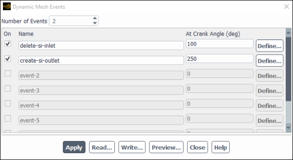
The procedure for defining events is as follows:
Increase the Number of Events value to the number of events you want to specify. As this value is increased, additional event entries in the dialog box will become editable.
Enable the check box next to the first event and enter a name for the event under the Name heading.
Specify either the time or the crank angle at which you want the event to occur.
For in-cylinder flows, specify the crank angle at which you want the event to occur under At Crank Angle.
For non-in-cylinder flows, specify the time (in seconds) at which you want the event to occur under At Time.
It is not necessary to specify the events in order of increasing time or crank angle, but it may be easier to keep track of events if you specify them in the order of increasing time or angle.
Click the button to open the Define Event Dialog Box (Figure 13.77: The Define Event Dialog Box).
In the Define Event Dialog Box, choose the type of event by selecting Change Zone Type, Copy Zone BC, Activate Cell Zone, Deactivate Cell Zone, Create Sliding Interface, Delete Sliding Interface, Change Motion Attribute, Change Time Step Size, Change Under-Relaxation Factors, Insert Boundary Zone Layer, Remove Boundary Zone Layer, Insert Interior Zone Layer, Remove Interior Zone Layer, Insert Cell Layer, Remove Cell Layer, Execute Command, Replace Mesh, Inert EGR Reset, or Diesel Unsteady Flamelet Reset in the Type drop-down list. These event types and their definitions are described later in this section.
Repeat steps 2–5 for the other events, if relevant.
Click Apply in the Dynamic Mesh Events Dialog Box after you finish defining all events.
To play the events to check that they are defined correctly, click the button in the Dynamic Mesh Events Dialog Box. This displays the Events Preview Dialog Box.
For in-cylinder flows, you use the Events Preview Dialog Box (Figure 13.78: The Events Preview Dialog Box for In-Cylinder Flows), to enter the crank angles at which you want to start and end the playback in the Start Crank Angle and End Crank Angle fields, respectively.
For non-in-cylinder flows, you use the Events Preview Dialog Box to enter the time at which you want to start and end the playback in the Start Time and End Time fields, respectively.
Specify the size of the step to take during the playback in the Increment field. Click Preview to play back the events. Ansys Fluent will play the events at the time (or crank angle in the case of in-cylinder flows) specified for each event and report when each event occurs in the text (console) window.
For in-cylinder simulations, you must specify the events for one complete engine cycle. In the subsequent cycles, the events are executed whenever

(13–30)
where
 is
the event crank angle,
is
the event crank angle,  is the current crank
angle calculated from Equation 13–26,
is the current crank
angle calculated from Equation 13–26,  is the crank angle period for one cycle, and
  is some integer.
As an example, for in-cylinder simulations, you are not required to specify the event crank angle to correspond exactly to the current crank angle calculated from Equation 13–26. Ansys Fluent will execute an event if the current crank angle is between
 where
where  is the equivalent change in crank angle for the time step. For example,
if the event preview is executed between crank angle of
is the equivalent change in crank angle for the time step. For example,
if the event preview is executed between crank angle of  and
and  (crank
period is
(crank
period is  ) using an increment
of
) using an increment
of  , Ansys Fluent will report the following
in the text window.
, Ansys Fluent will report the following
in the text window.Execute Event: open-in-valve-left (defined at: 353.10, current angle: 353.00) Execute Event: open-in-valve-right (defined at: 353.00, current angle: 353.00) Execute Event: close-ex-valve-right (defined at: 355.60, current angle: 356.00) Execute Event: close-ex-valve-left (defined at: 357.80, current angle: 358.00) Execute Event: close-in-valve-left (defined at: 571.60, current angle: 572.00) Execute Event: close-in-valve-right (defined at: 571.80, current angle: 572.00) Execute Event: open-ex-valve-right (defined at: 137.10, current angle: 857.00) Execute Event: open-ex-valve-left (defined at: 139.00, current angle: 859.00)
Notice that events defined at
 and
and  are executed at
  and
and  ,
respectively, because they satisfy the condition of Equation 13–30.
,
respectively, because they satisfy the condition of Equation 13–30.
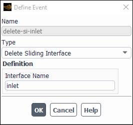
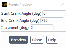
Ansys Fluent will automatically limit the valve lift values
depending on the specified minimum valve lift value. However, the
conversion of the sliding interface zones to walls (and vice versa)
is accomplished via the in-cylinder events (see Defining Dynamic Mesh Events). For example, if the exhaust
valve closes at  before
TDC position, you must define a Delete Sliding Interface event at the crank angle of
before
TDC position, you must define a Delete Sliding Interface event at the crank angle of  .
You must define similar events for the intake valve opening (using
the Create Sliding Interface event), the intake
valve closing (Delete Sliding Interface event),
and the exhaust valve opening (Create Sliding Interface event) at the respective crank angles.
.
You must define similar events for the intake valve opening (using
the Create Sliding Interface event), the intake
valve closing (Delete Sliding Interface event),
and the exhaust valve opening (Create Sliding Interface event) at the respective crank angles.
For the current example, the exhaust valve is assumed to be
open between  and
and  and the intake valve is open between at
  and
and  .
.
You can change the type of a zone to be a wall, or an interface, interior, fluid, or solid zone during your simulation. To change the type of a zone, select Change Zone Type in the Type drop-down list in the Define Event Dialog Box (Figure 13.77: The Define Event Dialog Box). Select the zone(s) that you want to change in the Zone list, and then select the new zone type in the New Zone Type drop-down list.
You can copy boundary conditions from one zone to other zones during your simulation. If, for example, you have changed an inlet zone to type wall with the Change Zone Type event, you can set the boundary conditions of the new zone type by simply copying the boundary conditions from a known zone with the corresponding zone type.
To copy boundary conditions from one zone to another, select Copy Zone BC in the Type drop-down list in the Define Event Dialog Box (Figure 13.77: The Define Event Dialog Box). In the From Zone drop-down list, select the zone that has the conditions you want to copy. In the To Zone(s) list, select the zone or zones to which you want to copy the conditions.
Ansys Fluent will set all of the boundary conditions for the zones selected in the To Zone(s) list to be the same as the conditions for the zone selected in the From Zone list. (You cannot copy a subset of the conditions, such as only the thermal conditions.)
Note that you cannot copy conditions from external walls to internal (that is, two-sided) walls, or vice versa, if the energy equation is being solved, since the thermal conditions for external and internal walls are different.
To activate a cell zone, select Activate Cell Zone in the Type drop-down list in the Define Event Dialog Box (Figure 13.77: The Define Event Dialog Box), then select the zone that you want to activate in the Zone(s) list. For more information, see Replacing, Deleting, Deactivating, and Activating Zones.
To deactivate a cell zone, select Deactivate Cell Zone in the Type drop-down list in the Define Event Dialog Box (Figure 13.77: The Define Event Dialog Box), then select the zone that you want to deactivate in the Zone(s) list.
Only deactivated zones can be activated. When a zone is deactivated, Ansys Fluent skips the zone during the calculations. For more information, see Replacing, Deleting, Deactivating, and Activating Zones.
To create a sliding interface during your simulation, select Create Sliding Interface in the Type drop-down list in the Define Event Dialog Box (Figure 13.79: The Define Event Dialog Box for the Creating Sliding Interface Option). Enter a name for the sliding interface in the Interface Name field. Select the zones on either side of the interface in the Interface Zone 1 and Interface Zone 2 drop-down lists.
You have the option to select any number of zones listed under each of the interface zones. Ansys Fluent calculates intersections between all possible combinations of the left and right side of the interfaces, allowing you more flexibility in terms of creating zones and defining the interfaces.
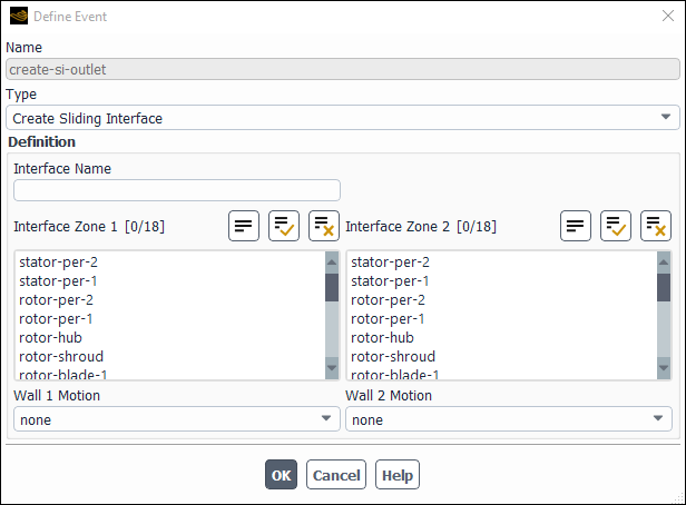
Important: If Ansys Fluent finds another interface with the same name as defined in the event, then the old interface will be deleted and a new one created as defined in the dynamic mesh event.
If the interface zones that you selected above do not overlap each other completely, the non-overlapped regions on each interface zones are put into separate wall zones by Ansys Fluent. If these wall zones (that is, non-overlapped regions) have motion attributes associated with them, their motion can only be specified by copying the motion from another dynamic zone by selecting the appropriate dynamic zones in the Wall 1 Motion and Wall 2 Motion drop-down lists, respectively.
Note that you do not have to change the boundary type from wall to interface. When the Create Sliding Interface event is executed, Ansys Fluent will automatically change the boundary type of the face zones selected in Interface Zone 1 and Interface Zone 2 to type interface before the sliding interface is created.
To delete a sliding interface that has been created earlier in your simulation, select Delete Sliding Interface in the Type drop-down list in the Define Event Dialog Box (Figure 13.77: The Define Event Dialog Box). Enter the name of the sliding interface to be deleted in the Interface Name field.
As with the Create Sliding Interface event, Ansys Fluent will automatically change the corresponding interface zones to wall. However, you may want to use the Copy Zone BC event to set any boundary conditions that are not the default conditions that Ansys Fluent assumes.
To change the motion attribute of a dynamic zone during your in-cylinder calculation, select Change Motion Attribute in the Type drop-down list in the Define Event Dialog Box (Figure 13.77: The Define Event Dialog Box). Select the Attribute (smoothing or remeshing) and set the appropriate Status (enable or disable). Select the corresponding dynamic zones for which you want to change the motion attributes in the Dynamic Zones list.
The smoothing attribute is used to enable or disable smoothing of nodes on selected deforming face zones and the remeshing attribute is used to enable and disable face remeshing on selected deforming face zones.
To change the time step size at some point during the simulation, select Change Time Step Size in the Type drop-down list in the Define Event Dialog Box. Specify the new physical time step size by entering the new Time Step Size in seconds.
For in-cylinder simulations, specify the new physical time step size by entering the new Crank Angle Step Size value in degrees. The physical time step size is calculated from
 | (13–31) |
To change one or more under-relaxation factors, select Change Under-Relaxation Factor in the Type drop-down list in the Define Event Dialog Box (Figure 13.77: The Define Event Dialog Box). Select the under-relaxation factor that you want to change, and assign a new value to it in the Under-Relaxation Factors list. For more information on setting under-relaxation factors, see Setting Under-Relaxation Factors.
To insert a new cell zone layer as a separate cell zone adjacent to a boundary, select Insert Boundary Zone Layer in the Type drop-down list in the Define Event Dialog Box. Specify the Base Dynamic Zone, from which the layer of cells is to be created, and the Side Dynamic Zone, which represents the deforming face zone adjacent to the Base Dynamic Zone before the layer is inserted. The new cell zone will inherit the boundary conditions of the cell zone adjacent to the Base Dynamic Zone before the layer is inserted.
Note that a new cell layer can be inserted only from a one-sided Base Dynamic Zone. You cannot insert a new cell layer from an interior face zone.
Figure 13.80: Boundary Zone Before Insertion and Figure 13.81: Boundary Zone After Insertion illustrate the insertion of a boundary zone layer. In both figures, the circular face at the top of the cylinder is the base dynamic zone.
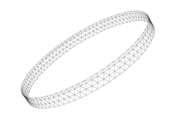
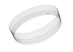
To remove the cell zone layer inserted using the Insert Boundary Zone Layer event, select Remove Boundary Zone Layer in the Type drop-down list in the Define Event Dialog Box. Specify the same Base Dynamic Zone that you used when you defined the insert boundary layer event.
Note that a cell layer can be removed only from a one-sided Base Dynamic Zone.
To insert a new zone layer as a separate cell zone adjacent to the internal side of a boundary, select Insert Interior Zone Layer in the Type drop-down list in the Define Event Dialog Box. Specify the Base Dynamic Zone and the Side Dynamic Zone as described in the Insert Boundary Zone Layer event. You also must specify the names of the new interior face zones (Internal Zone 1 Name and Internal Zone 2 Name) that will be created after the cell zone layer is created by Ansys Fluent.
Ansys Fluent inserts the interior cell layer by splitting the cell zone adjacent to the Base Dynamic Zone with a plane. The position of the plane and the normal direction of the plane are implicitly defined by the cylinder origin and cylinder axis of the Side Dynamic Zone.
Figure 13.82: Interior Zone Before Insertion and Figure 13.83: Interior Zone After Insertion illustrate the insertion of an interior zone layer.

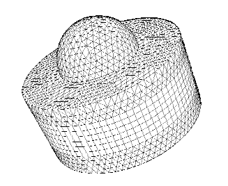
To remove the zone layer inserted using the Insert Interior Zone Layer event, select Remove Interior Zone Layer in the Type drop-down list in the Define Event Dialog Box. Specify the same Internal Zone 1 Name and Internal Zone 2 Name that you used to define the Insert Interior Zone Layer event.
To manually insert a new cell layer to the existing cell zone, select Insert Cell Layer in the Type drop-down list in the Define Event Dialog Box. Specify the Adjacent Dynamic Face Zone and the Direction Parameter. This can only work on zones that are suited for layering (see Applicability of the Dynamic Layering Method).
To manually remove a cell layer from an existing cell zone, select Remove Cell Layer in the Type drop-down list in the Define Event Dialog Box. Specify the Adjacent Dynamic Face Zone and the Direction Parameter. This can only work on zones that are suited for layering (see Applicability of the Dynamic Layering Method).
To execute a command, select Execute Command in the Type drop-down list in the Define Event Dialog Box (Figure 13.77: The Define Event Dialog Box). A command can be a series of text or Scheme commands, or a macro you have defined (or will define) using the Define Macro Dialog Box (see Defining Macros). Enter the series of commands or the name of the macro in the Command text-entry box.
Important: If the command to be executed involves saving a file, see Saving Files During the Calculation for important information.
To replace the mesh and interpolate existing data onto the new mesh during your simulation, select Replace Mesh from the Type drop-down list in the Define Event dialog box (Figure 13.77: The Define Event Dialog Box). Then, specify the replacement mesh under Mesh File. Enable Interpolate Data Across Zones if necessary (see Replacing the Mesh for details).
To convert burnt gases at the end of the cycle to inert for the next cycle, select Inert EGR Reset from the Type drop-down list in the Define Event dialog box (Figure 13.77: The Define Event Dialog Box). Specify the Zone(s). For further details, see Resetting Inert EGR.
To simulate multiple-cycle internal combustion engines using diesel unsteady flamelets, select Diesel Unsteady Flamelet Reset from the Type drop-down list in the Define Event dialog box (Figure 13.77: The Define Event Dialog Box). Specify the Zone(s). This event is only applicable to and available with diesel unsteady flamelets with two or more flamelets. For further details, see Resetting Diesel Unsteady Flamelets. Note that Diesel Unsteady Flamelet Reset is generally preferable to Inert EGR Reset since an additional transport equation is avoided.
If you want to save the events you have defined to a file, click in the Dynamic Mesh Events Dialog Box and specify the Event File in The Select File Dialog Box.
To read the events back into Ansys Fluent, click in the Dynamic Mesh Events Dialog Box and specify the Event File in The Select File Dialog Box.
You must define the motion of the dynamic zones in your model. If the zone is a rigid body, you can use a motion definition, profile, or user-defined function (UDF) to define the motion of the rigid body, or use the six DOF solver. If the zone is a deforming zone, you can define the geometry and the parameters that control the face or zone remeshing, if applicable. For a zone that is deforming and moving at the same time, you can use a user-defined function to define the geometry and motion of the zone as they change with time.
You will specify the motion of the dynamic zones in your model using the Dynamic Mesh Zones dialog box
![]() Setup →
Setup → ![]() Dynamic
Mesh → Create/Edit...
Dynamic
Mesh → Create/Edit...
Details about specifying different types of motion are provided in this section.
When you have completed the specification of a dynamic zone, click in the Dynamic Mesh Zones Dialog Box to complete the specification and add the zone to the Dynamic Mesh Zones list.
If you want to make a change to the specification of a dynamic zone, double-click the zone in the Dynamic Mesh Zones list, change the specification, and then click in the Dynamic Mesh Zones Dialog Box to update the specification.
If a dynamic zone has rigid body motion, you can view its current position and orientation of the center of gravity (with respect to initial data) by double-clicking the zone in the Dynamic Mesh Zones list and viewing the values under Center of Gravity Location and Rigid Body Orientation.
By default, if no motion (moving or deforming) attributes are assigned to a face or cell zone, then the zone is not considered when updating the mesh to the next time step. However, there are cases where an explicit declaration of a stationary zone is required. For example, if a cell zone is assigned some solid body motion, the positions of all nodes belonging to the cell zone will be updated even though some of the nodes may also be part of a non-moving boundary zone. An explicit declaration of a stationary zone excludes the nodes on these zones when updating the node positions.
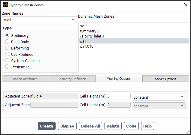
To define a stationary zone in your model, follow the steps below.
Select the stationary zone in the Zone Names drop-down list.
Select Stationary under Type.
If the stationary zone is a face zone, then define the Cell Height in the Meshing Options tab for any Adjacent Zone that is involved in dynamic layering. It does not influence the cell size for local or global remeshing. The Cell Height specifies the ideal height (
 in Equation 13–15 and Equation 13–16 of the adjacent cells. Make a selection in
the Cell Height drop-down menu to specify this value as either a
constant or a compiled user-defined function.
in Equation 13–15 and Equation 13–16 of the adjacent cells. Make a selection in
the Cell Height drop-down menu to specify this value as either a
constant or a compiled user-defined function.If you select the constant option, enter a value in the Cell Height text-entry box.
If you choose to use a compiled user-defined function to define an ideal cell height that varies as a function of time or crank angle, you must first define a
DEFINE_DYNAMIC_ZONE_PROPERTYUDF. After you have compiled the UDF source file, built a shared library, and loaded it into Ansys Fluent, the name of the UDF library will be available for selection in the Cell Height drop-down list.Refer to the Fluent Customization Manual for information about UDFs.
For cases with strong fluid-structure interaction, solution stabilization may help convergence for boundary zones. Solution stabilization can be set in the Solver Options tab. See Solution Stabilization for Dynamic Mesh Boundary Zones for details.
Click Create.
To define a rigid-body zone in your model, follow the steps below.
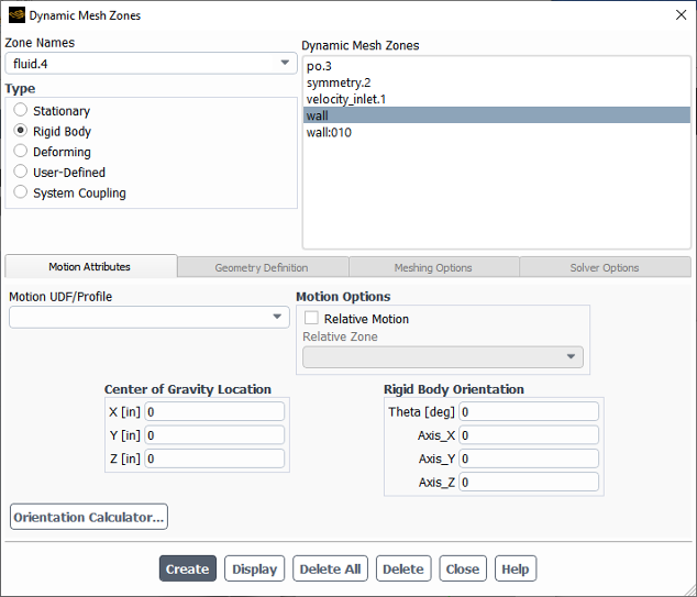
Select the rigid body zone in the Zone Names drop-down list.
Select the Rigid Body option under Type.
If you want to specify the motion of the rigid body zone using a motion definition, profile, or user-defined function, then make a selection from the Motion UDF/Profile drop-down list in the Motion Attributes tab. Note that the names of motion definitions are preceded by motion:: in this list. See Managing Motion Definitions for information about motion definitions, see Profiles and Solid-Body Kinematics for information on profiles, and see the Fluent Customization Manual for information on user-defined functions. Using a motion definition may be advantageous, as it can be simpler to set up and allows you to use expressions to define the rigid body motion.
If you enabled the In-Cylinder option in the Dynamic Mesh Task Page, Ansys Fluent provides built-in functions in the Motion UDF/Profile drop-down list that can be useful for defining the rigid body motion of a piston. If you would like the motion of the piston to be a function of crank angle (that is, governed by Equation 13–25), then you should select **piston-full**. For further information, see In-Cylinder Settings.
If you enabled the Six DOF option in the Dynamic Mesh Task Page, make sure that On is enabled in the Six DOF group box in the Motion Attributes tab (see Figure 13.87: The Dynamic Mesh Zones Dialog Box for a Rigid Body Motion Using the Six DOF Solver), to ensure that the six DOF solver is being used. Then make a selection from the Six DOF UDF/Properties drop-down list; for details on creating the selections available in this list, Setting Rigid Body Motion Attributes for the Six DOF Solver.
Note that the Passive option in the Six DOF group box is used when you do not want the forces and moments on the zone to be taken into consideration.
Specify the initial location of the center of gravity for the rigid body by entering coordinates in the Center of Gravity Location group box.
If you want a rigid body to move relative to another rigid body, then you must enable Relative Motion and specify the Relative Zone.
Note: You must create the relative rigid body zone before creating a rigid body that is dependent on that zone, if you are setting up the motion using the graphical user interface (GUI). The order in which you specify the zones does not matter if you set up the motion using the text user interface (TUI).
Specify the orientation of the rigid body in Rigid Body Orientation. You can consider the orientation of the rigid body as the rotation that it would take to rotate the global coordinate system into your desired rigid body coordinate system. For most cases, you will use these fields as a way to keep track of the object’s current orientation, as Ansys Fluent will update your initial rigid body orientation values as the calculation progresses. The rigid body orientation is used, if needed, by the six DOF solver to evaluate the external load forces and moments (see
DEFINE_SDOF_PROPERTIESin the Fluent Customization Manual), as well as when evaluating the relative motion of a dynamic zone with respect to another (seeDEFINE_CG_MOTIONin the Fluent Customization Manual).The orientation is expressed in the axis angle format. Per the Euler Theorem, any set of rotations around a fixed point can be expressed via a single rotation about a specific axis. If you know the orientation of the rigid body in another format or as a set of consecutive rotations, you can use the Orientation Calculator dialog box and evaluate the equivalent axis angle format. To open this dialog box, click the button; then you can perform the following steps:
Enter a value, either in Axis and Angle, Rotation Matrix, or Euler Angle format, and click to see the value in the output format.
The calculator also converts the entered values into the other two “grayed-out” input formats.
Note: There are several possible Euler angle representations. Fluent uses a vector defined by
 ,
,  , and
, and  where:
  is the rotation about the original Z axis,
  is the rotation about the rotated Y axis, and
  is the rotation about the rotated X axis.
Enable Concatenate Next Input if you want the next input to be concatenated to the previous output.
Click to use the current Output as your Rigid Body Orientation in the Dynamic Mesh Zones dialog box.
When using the six DOF solver, specify the velocity of the center of gravity with respect to the global coordinate system by entering the velocity of the center of gravity in Center of Gravity Velocity. Also, specify the angular velocity of the rigid body with respect to the global coordinate system by entering the angular velocity of the rigid body in Rigid Body Angular Velocity. Note that these fields are ignored for one DOF rotation and translation, respectively.
If you are solving an in-cylinder problem, specify the direction of the reference axis of the valves or piston in Valve/Piston Axis.
The current valve lift or piston stroke is automatically updated in Lift/Stroke when you click based on the parameters you have specified earlier when you first invoke the in-cylinder option.
By default, the boundary mesh motion is taken into consideration when imposing the physical boundary conditions, even if the boundary moves because of a moving adjacent cell zone and no dynamic zone has been created for the boundary. If this is not the desired behavior and you instead want to exclude the mesh motion from contributing to the boundary conditions, then you need to enable the Exclude Mesh Motion in Boundary Conditions option for that boundary zone in the Motion Attributes tab.
If the rigid body zone is a face zone, specify the Cell Height for each Adjacent Zone in the Meshing Options tab. The Cell Height is the ideal cell height (
 in Equation 13–15 and Equation 13–16 that is used by Ansys Fluent to determine
when the prismatic layer next to the rigid body should be split or merged with the layer next
to it. If the adjacent zone is tetrahedral or triangular, the ideal height is used by
Ansys Fluent to determine if adjacent cells must be agglomerated for local remeshing. Make a
selection in the Cell Height drop-down menu to specify this value as
either a constant or a compiled user-defined function.
in Equation 13–15 and Equation 13–16 that is used by Ansys Fluent to determine
when the prismatic layer next to the rigid body should be split or merged with the layer next
to it. If the adjacent zone is tetrahedral or triangular, the ideal height is used by
Ansys Fluent to determine if adjacent cells must be agglomerated for local remeshing. Make a
selection in the Cell Height drop-down menu to specify this value as
either a constant or a compiled user-defined function.If you select the constant option, enter a value in the Cell Height text-entry box.
If you choose to use a compiled user-defined function to define an ideal cell height that varies as a function of time or crank angle, you must first define a
DEFINE_DYNAMIC_ZONE_PROPERTYUDF. After you have compiled the UDF source file, built a shared library, and loaded it into Ansys Fluent, the name of the UDF library will be available for selection in the Cell Height drop-down list.Refer to the Fluent Customization Manual for information about UDFs.
If the dynamic zone is a face zone with an adjacent boundary layer mesh, you must apply boundary layer smoothing using the Deform Adjacent Boundary Layer with Zone option in the Meshing Options tab if you want the boundary layer to move with the moving face zone. For example, this option is necessary if you are applying face region remeshing with prism layers and you have not decomposed the mesh volume (see Face Region Remeshing with Wedge Cells in Prism Layers). In such circumstances, the Deform Adjacent Boundary Layer with Zone option ensures that the base prism elements shown in Figure 13.45: Volume Decomposition for the Base of the Prism Layers will move rigidly with the piston.
Note that the boundary layer smoothing method is primarily intended for translational motion of the face zone. If significant rotation is applied to the face zone, the boundary layer cells may become skewed. For more information refer to Boundary Layer Smoothing Method.
For cases with strong fluid-structure interaction, solution stabilization may be necessary for boundary zones if the use of implicit mesh updating (described in Implicit Update Settings) is insufficient to stabilize the solver due to the fluid motion. Solution stabilization options can be set in the Solver Options tab. See Solution Stabilization for Dynamic Mesh Boundary Zones for details.
Click Create.
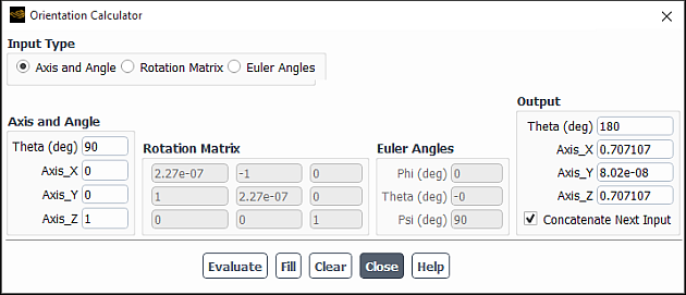
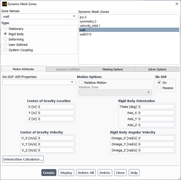
To define a deforming zone in your model, follow the steps below.
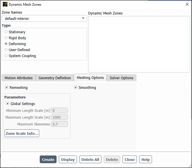
Select the deforming zone in the Zone Names drop-down list.
Select the Deforming option under Type.
By default, the boundary mesh motion is not taken into consideration when imposing the physical boundary conditions. If this is not the desired behavior and you instead want to include the mesh motion in the boundary conditions, then you need to disable the Exclude Mesh Motion in Boundary Conditions option for that boundary zone in the Motion Attributes tab. For example, you might want to disable this option when using the linearly elastic solid mesh smoothing method with the unspecified geometry option to not only smooth the mesh but to also propagate the motion from another boundary.
Specify the geometry of the deforming zone in the Geometry Definition tab.
If no geometry is available, select faceted in the Definition drop-down list.
If the geometry is a plane, select plane in the Definition drop-down list. To define the plane, enter the position of a point on the plane in Point on Plane and the plane normal in Plane Normal.
If the geometry is a cylinder, select cylinder in the Definition drop-down list. To define the cylinder, enter the Cylinder Radius, the Cylinder Origin and the Cylinder Axis.
If the geometry is unspecified and mesh motion normal to the boundary is permissible, select unspecified in the drop-down list. This option is only available if the linearly elastic solid mesh smoothing method or the radial basis function smoothing method is enabled (see Linearly Elastic Solid Based Smoothing Method or Radial Basis Function Smoothing, respectively). Note that with the radial basis function smoothing method, if you have a non-conformal interface where both of the interface boundaries are deforming dynamic zones with unspecified geometry, then Fluent will ensure that the two interface zones stay connected (by projecting one of the interface zones onto the other); such behavior is only supported if the same cell zone is on either side of the non-conformal interface.
If the geometry is described by a user-defined function, select user-defined in the Definition drop-down list and the appropriate user-defined functions in the Geometry UDF drop-down list. See the Fluent Customization Manual for information on user-defined functions.
If the geometry is defined by an auxiliary geometry definition that you have created previously (for details, see Managing Auxiliary Geometry Definitions), select it in the Definition drop-down list. The names of auxiliary geometry definitions are preceded by geom:: in this list, in order to identify them.
Note: Auxiliary geometry definitions of the Reconstruction type are not available for selection when Remeshing is enabled in the Mesh Methods list in the Dynamic Mesh task page.
For 3D simulations, Ansys Fluent allows you to preserve features on the boundary zones that are important for the flow. Such features may be at the juncture of different boundary zones, or they may be on a single non-planar boundary zone. For any geometry definition (faceted, plane, cylinder, or user-defined), you can indicate whether you want to preserve features of a specific angular range by enabling Feature Detection under Feature Options and setting a threshold value for the Feature Angle in degrees. For more information (including how the Feature Angle is defined), see Feature Detection.
When available, the geometry information is used to project nodes on the deforming zone after remeshing the face zone, or if nodes are moved through smoothing.
For deforming boundary and cell zones, specify the appropriate remeshing parameters in the Meshing Options tab.
You can locally enable Remeshing and define the settings in the group box under this option, including the following:
Under Parameters, enabling the Global Settings option ensures that settings defined in the Mesh Method Settings Dialog Box are used for this dynamic zone. Disabling this option allows you to revise the Minimum Length Scale, Maximum Length Scale and/or Maximum Skewness locally. When setting these values, you should use the vital statistics of your zone found in the Zone Scale Info Dialog Box, which can be opened by clicking the button.
For boundary zones, you may have additional Options: if you selected Methods-Based Remeshing in the Mesh Method Settings Dialog Box, you can specify the remeshing methods applied to this dynamic zone, including Region and Local.
You can locally enable Smoothing and, if Spring/Laplace/Boundary Layer is selected for smoothing in the Mesh Method Settings Dialog Box, define the settings in the group box under this option, including the following:
If you selected a cell zone, enabling the Global Settings option ensures that the element type defined in the Mesh Smoothing Parameters Dialog Box is used for this dynamic zone. Disabling it allows you to select a different element type locally.
If you selected a boundary zone, you can specify whether the smoothing method is spring based or Laplacian.
For cases with strong fluid-structure interaction, solution stabilization may help convergence for boundary zones. Solution stabilization can be set in the Solver Options tab. See Solution Stabilization for Dynamic Mesh Boundary Zones for details.
Click Create.
For a zone that is deforming and/or moving, you can define the position of each node on the general deforming / moving zone using a user-defined function (UDF). To define a moving / deforming zone, follow the steps below.
Select the moving and deforming zone in the Zone Names drop-down list.
Select the User-Defined option under Type.
In the Motion Attributes tab, select the user-defined function that defines the geometry and motion of the zone from the Mesh Motion UDF/Profile drop-down list. See the Fluent Customization Manual for information on user-defined functions used to specify user-defined motion.
By default, the boundary mesh motion is taken into consideration when imposing the physical boundary conditions. If this behavior is not desired and you instead want to exclude the mesh motion from contributing to the boundary conditions, then you need to enable the Exclude Mesh Motion in Boundary Conditions option for that boundary zone in the Motion Attributes tab. The following are examples of when you might want to exclude such motion:
You have created a dynamic zone for a cell zone that moves, but one or more of the boundaries of that cell zone should be treated as stationary.
You are using a
DEFINE_GRID_MOTIONUDF that defines nodal motion on a boundary that, for example, includes both rigid body motion (which should contribute to the boundary condition) and smoothing (which should not). With such UDFs, you must perform the following steps for that boundary:Enable the Exclude Mesh Motion in Boundary Conditions option.
Define the rigid body motion in the Momentum tab of the Wall dialog box.
If you want the movement / deformation to be relative to the rigid body motion of a cell zone, then you can enable Relative Motion and select the cell zone from the Relative Zone list.
Note: You must specify the movement / deformation in your UDF using
NODE_COORD_NEST, rather than specify the final coordinates (as you would if you were NOT specifying it relative to a cell zone). For additional information, seeDEFINE_GRID_MOTIONin the Fluent Customization Manual.You must create the relative rigid body zone before creating the user-defined zone if you are setting up the zones using the graphical user interface (GUI). The order in which you create the zones does not matter if you set up the zones using the text user interface (TUI).
For a face zone, you can specify the Cell Height in the Meshing Options tab for any Adjacent Zone that is involved in local remeshing or dynamic layering. The Cell Height specifies the ideal height (
 in Equation 13–15 and Equation 13–16 of the adjacent cells. Make a selection in
the Cell Height drop-down menu to specify this value as either a
constant or a compiled user-defined function.
in Equation 13–15 and Equation 13–16 of the adjacent cells. Make a selection in
the Cell Height drop-down menu to specify this value as either a
constant or a compiled user-defined function.If you select the constant option, enter a value in the Cell Height text-entry box.
If you choose to use a compiled user-defined function to define an ideal cell height that varies as a function of time or crank angle, you must first define a
DEFINE_DYNAMIC_ZONE_PROPERTYUDF. After you have compiled the UDF source file, built a shared library, and loaded it into Ansys Fluent, the name of the UDF library will be available for selection in the Cell Height drop-down list.Refer to the separate Fluent Customization Manual for information about UDFs.
If the dynamic zone is a face zone with an adjacent boundary layer mesh, and you want to use the boundary layer smoothing method (as described in Boundary Layer Smoothing Method), enable the Deform Adjacent Boundary Layer with Zone option in the Meshing Options tab.
For a 3D boundary zone, you can allow local face remeshing by enabling the Local option (under Remeshing Method) in the Meshing Options tab. For details, see Local Face Remeshing Method. Enabling this option allows you to do the following:
You can revise the Maximum Skewness allowed for faces if you want to specify a local value for this dynamic zone that differs from the one you specified globally in the Mesh Method Settings Dialog Box. Note that the global setting may still be used if Ansys Fluent determines that your local setting is unreasonable.
You can preserve features, not only at the juncture of different boundary zones, but also on a single non-planar boundary zone. In the Geometry Definition tab, you can indicate whether you want to include features of a specific angular range by enabling Feature Detection under Feature Options and setting a threshold value for the Feature Angle in degrees. For more information (including how the Feature Angle is defined), see Feature Detection.
For cases with strong fluid-structure interaction, solution stabilization may help convergence for boundary zones. Solution stabilization can be set in the Solver Options tab. See Solution Stabilization for Dynamic Mesh Boundary Zones for details.
Click Create.
If this zone is part of a mesh interface and only one side undergoes user-defined motion, then by default that motion will be transferred to the other side in order to maintain the coupling. You can change the method by which the displacement of the passive nodes is calculated or disable this transfer altogether, as described in Transferring Motion Across a Mesh Interface.
For a boundary layer that deforms according to the adjacent face zone, the zone that is deforming and moving is usually defined using a user-defined function (UDF), as described in User-Defined Motion. To define a moving and deforming boundary layer, perform the steps that follow.
If the boundary layer borders a face zone that is only moving and is not deforming, you should consider applying rigid body motion to the face zone (see Rigid Body Motion) rather than user-defined motion, as rigid body motion usually involves a simpler definition.
Set up the moving and deforming zone.
Select the moving and deforming zone in the Zone Names drop-down list.
Select User-Defined from the Type list.
In the Motion Attributes tab, select the user-defined function that defines the geometry and motion of the zone from the Mesh Motion UDF/Profile drop-down list.
In the Meshing Options tab, enable the Deform Adjacent Boundary Layer with Zone option.
Click Create.
Set up a deforming dynamic zone for the fluid zone that contains the boundary layer.
Select the fluid zone that contains the boundary layer from the Zone Names drop-down list.
Select Deforming from the Type list.
In the Meshing Options tab, ensure that Remeshing and Smoothing are enabled.
Click Create.
If the fluid zone set up in the step 2 consists entirely of the boundary layer elements, set up a deforming dynamic zone for the neighboring fluid zone. This step is necessary because the deforming boundary layer will deform the adjacent cells.
Select the fluid zone that neighbors the boundary layer zone from the Zone Names drop-down list.
Select Deforming from Type list.
In the Meshing Options tab, enable Smoothing and Remeshing in the Methods group box.
Click Create.
For a zone that is involved in a system coupling, the motion is defined by the application that Ansys Fluent is coupled with on this zone. For more details about setting up a simulation with system coupling see Performing System Coupling Simulations Using Fluent and the System Coupling User's Guide. To define a system coupling region, follow the steps below.
Select the moving and deforming zone in the Zone Names drop-down list.
Select the System Coupling option under Type.
You must specify the Cell Height in the Meshing Options tab for any Adjacent Zone that is involved in local remeshing or dynamic layering. The Cell Height specifies the ideal height (
 in Equation 13–15 and Equation 13–16 of the adjacent cells. Make a selection in
the Cell Height drop-down menu to specify this value as either a
constant or a compiled user-defined function.
in Equation 13–15 and Equation 13–16 of the adjacent cells. Make a selection in
the Cell Height drop-down menu to specify this value as either a
constant or a compiled user-defined function.If you select the constant option, enter a value in the Cell Height text-entry box.
If you choose to use a compiled user-defined function to define an ideal cell height that varies as a function of time or crank angle, you must first define a
DEFINE_DYNAMIC_ZONE_PROPERTYUDF. After you have compiled the UDF source file, built a shared library, and loaded it into Ansys Fluent, the name of the UDF library will be available for selection in the Cell Height drop-down list.Refer to the separate Fluent Customization Manual for information about UDFs.
For cases with strong fluid-structure interaction, solution stabilization may be necessary to achieve convergence for boundary zones undergoing system coupling motion. Solution stabilization options can be set in the Solver Options tab. See Solution Stabilization for Dynamic Mesh Boundary Zones for details.
Click Create.
If this zone is part of a mesh interface and only one side undergoes system coupling motion, then by default that motion will be transferred to the other side in order to maintain the coupling. You can change the method by which the displacement of the passive nodes is calculated or disable this transfer altogether, as described in Transferring Motion Across a Mesh Interface.
Note: If the System Coupling option is enabled, and Ansys Fluent is not involved with a system coupling simulation, then this zone type behaves in the same way as a stationary zone.
For a two-way intrinsic fluid-structure interaction (FSI) simulation, you can specify that a wall zone between a fluid and solid cell zone deforms according to the deformation of the adjacent solid zone by performing the following steps. For more details about setting up an intrinsic FSI simulation, see Setting Up an Intrinsic Fluid-Structure Interaction (FSI) Simulation.
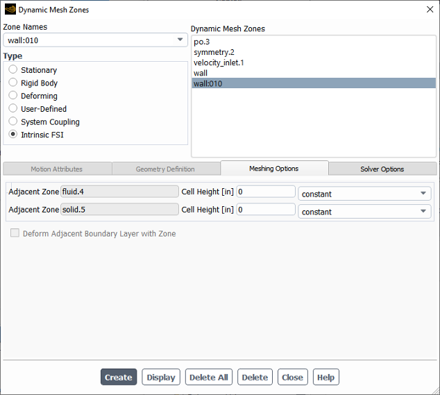
Select a wall zone that is between a fluid and solid cell zone in the Zone Names drop-down list. Note that this zone must be the side of a two-sided wall (that is, the wall or wall-shadow) that is immediately adjacent to the fluid cell zone (as indicated by the Adjacent Cell Zone field in the Wall dialog box).
Select Intrinsic FSI from the Type list. Note that this type is only available when you have selected a model in the Structural Model Dialog Box.
For a face zone, you can specify the Cell Height in the Meshing Options tab for any Adjacent Zone that is involved in local remeshing or dynamic layering. The Cell Height specifies the ideal height (
in Equation 13–15 and Equation 13–16 of the adjacent cells. Make a selection in
the Cell Height drop-down menu to specify this value as either a
constant or a compiled user-defined function.If you select the constant option, enter a value in the Cell Height text-entry box.
If you choose to use a compiled user-defined function to define an ideal cell height that varies as a function of time or crank angle, you must first define a
DEFINE_DYNAMIC_ZONE_PROPERTYUDF. After you have compiled the UDF source file, built a shared library, and loaded it into Ansys Fluent, the name of the UDF library will be available for selection in the Cell Height drop-down list.Refer to the separate Fluent Customization Manual for information about UDFs.
If the dynamic zone is a face zone with an adjacent boundary layer mesh, and you want to use the boundary layer smoothing method (as described in Boundary Layer Smoothing Method), enable the Deform Adjacent Boundary Layer with Zone option in the Meshing Options tab.
For cases with strong fluid-structure interaction, solution stabilization may help convergence for boundary zones. Solution stabilization can be set in the Solver Options tab. See Solution Stabilization for Dynamic Mesh Boundary Zones for details.
Click Create.
For cases with strong fluid-structure interaction, stabilization is achieved through a boundary source coefficient introduced in the continuity equation, designed to improve the diagonal dominance of the matrix system in the cells adjacent to dynamic mesh boundary zones. Two methods for this boundary source coefficient are available:
volume-based
This method uses the cell volume
 to re-scale the diagonal entry of the linear matrix system corresponding to
the discretized continuity equation (
to re-scale the diagonal entry of the linear matrix system corresponding to
the discretized continuity equation ( ) as
) as  :
: 
(13–32)
coefficient-based
This method directly re-scales the diagonal entry of the linear matrix system corresponding to the discretized continuity equation (
 ) as
) as  :
:
(13–33)
where  is the scale factor and
  is the number of cells. Note that the value you choose for
  will only affect the rate of convergence, and will not affect the converged
solution.
will only affect the rate of convergence, and will not affect the converged
solution.
Note: While solution stabilization is available for all types of dynamic mesh boundary zones, it is more commonly needed for rigid body motion with the six degrees of freedom (six DOF) solver or for system coupling motion. It is not recommended for boundary zones of type interior, as it can adversely affect convergence.
Solution stabilization can be enabled for a boundary zone by opening the Solver
Options tab in the Dynamic Mesh Zones Dialog Box, enabling the
Solution Stabilization option, and then defining the settings under
Stabilization Parameters. Available settings include the Scale
Factor () and the Method, which can be either
volume-based or coefficient-based (default). The
Scale Factor must be set to a nonzero value for the stabilization to have
an effect.
The solver option settings can also be defined using the
define/dynamic-mesh/zones/create text command, and a summary of these
settings can be printed in the console for each dynamic zone by using the
define/dynamic-mesh/zones/list text command.
Ansys Fluent uses solid-body kinematics if the motion is prescribed based on the position and orientation of the center of gravity of a moving object. This is applicable to both cell and face zones.
The motion of the solid-body can be specified either as a profile or as a user-defined function (UDF). A profile may be defined by the following profile fields:
time (time)
crank angle (angle) (in-cylinder flows only)
position (
 ,
,  ,
,  )
)linear velocity (
 ,
,  ,
,  )
)angular velocity (
 ,
,  ,
,  )
)orientation (
 ,
,  ,
,  )
)
For in-cylinder simulations, the velocity profiles for valves can be expressed as a function of crank angle instead of time. In addition, transient boundary condition profiles can also be expressed as a function of crank angle instead of time. For more information about transient profiles, see Transient Cell Zone and Boundary Conditions.
Below are two examples of a profile format:
 ((movement_linear 3 point)
 (time
 0  1  2 )
 (x
 2  3  4 )
 (v_y
 0  -5  0 )
 )
 ((movement_angular 3 point)
 (time
 0  1  2 )
 (omega_x
 2  3  4 )
 )
For in-cylinder flows, crank angles can be included in transient tables as well as transient profiles, in a similar fashion to time. An example of a transient table using (crank) angle is as follows:
 example 2 3 1
 angle temperature
 0  300
 180 500
 360 300
An example of a transient profile using (crank) angle is as follows:
 ((example transient 3 1)
 (angle
 0.000000e+00 1.800000e+02 3.600000e+02)
 (temperature
 3.000000e+02 5.000000e+02 3.000000e+02)
 )
In addition to the motion description, you must also specify the starting location of the center of gravity and orientation of the solid body. In 2D cases (and 3D cases that do not use the six DOF solver), Ansys Fluent automatically updates the center of gravity position and orientation at every time step such that
 | (13–34) |
where  and
and  are the position and orientation of the center of gravity,
  and
and  are the linear and angular velocities of the center of gravity. 3D, six DOF
cases use a more complex form of Equation 13–34 when updating
are the linear and angular velocities of the center of gravity. 3D, six DOF
cases use a more complex form of Equation 13–34 when updating
 .
.
Typically,  is chosen to be an appropriate set of Euler angles. In this case, the
solid-body motion must be specified using a user-defined function
(
is chosen to be an appropriate set of Euler angles. In this case, the
solid-body motion must be specified using a user-defined function
(DEFINE_CG_MOTION).
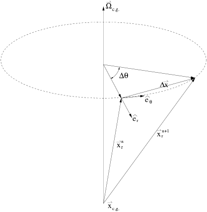
The position vectors on the solid body are updated based on rotation about the
instantaneous angular velocity vector  . For a finite rotation angle
  =
=  , the final position of a vector
  on the solid body with respect to
  can be expressed as (See Figure 13.90: Solid Body Rotation Coordinates)
 | (13–35) |
where  can be shown to be
 | (13–36) |
The unit vectors  and
and  are defined as
 | (13–37) |
 | (13–38) |
If the solid body is also translating with  , the
, the  position vector on the solid body can be expressed as
 | (13–39) |
where  is given by Equation 13–35.
When you have specified the mesh update methods and their associated parameters, and you have defined the motion of dynamic zones, as described in Specifying the Motion of Dynamic Zones, you can preview the motion of the mesh or the zone as it changes with time before you start your simulation. The same dynamic zone or mesh motion will be executed when you start your simulation.
You can preview the motion of zones with Rigid Body or User-Defined motion using the Zone Motion Dialog Box (Figure 13.91: The Zone Motion Dialog Box).
![]() Setup →
Setup → ![]() Dynamic Mesh → Display Zone Motion...
Dynamic Mesh → Display Zone Motion...
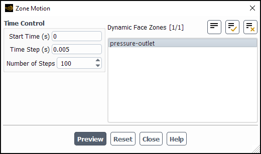
The zone motion preview only updates the graphical representation (in the graphics window) of the zones that you have selected in the Dynamic Face Zones list. Only zones that have been specified with either User-Defined or Rigid Body motion type are available for zone motion preview. To use the Zone Motion preview:
In the Zone Motion Dialog Box, select the face zones for which you want to preview the motion from the Dynamic Face Zones list. The Dynamic Face Zones list displays zones that have either User-Defined or Rigid Body motion specified. By default, all such zones are selected.
Enter the Start Time, Time Step, and Number of Steps under Time Control.
Click the button to preview the zone motion. This positions the mesh according to the specified Start Time, and then integrates the position of the selected surfaces in time. The zone positions at the specified Start Time can be previewed without any subsequent motion by entering 0 for the Number of Steps.
Click Reset to restore the mesh to its initial state.
Previewing the zone motion can also be used as a postprocessor for six DOF simulations (see Six DOF Solver Settings).
The mesh motion preview is different from the zone motion described above in that the mesh connectivity is changed in mesh motion.
To preview the dynamic mesh of a transient case, you can use the Mesh Motion Dialog Box (Figure 13.92: The Mesh Motion Dialog Box)
![]() Setup →
Setup → ![]() Dynamic Mesh → Preview Mesh Motion...
Dynamic Mesh → Preview Mesh Motion...
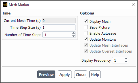
The procedure is as follows:
Save the case file.
File → Write → Case...
Important: Note that the mesh motion will actually update the node locations as well as the connectivity of the mesh, so you must be sure to save your case file before doing the dynamic mesh motion. Once you have advanced the mesh by a certain number of time steps, you will not be able to recover the previous status of the mesh, other than by reloading the appropriate Ansys Fluent case file.
Specify the Number of Time Steps and the size of each time step (Time Step Size). The current time will be displayed in the Current Mesh Time field after the dynamic mesh has been advanced the specified number of steps.
Note that if you turned on the in-cylinder option, the Time Step Size is automatically calculated from the Crank Angle Step Size and the Crank Shaft Speed that you have specified in the In-Cylinder tab of the Options Dialog Box.
To view the dynamic mesh in the graphics window, enable the Display Mesh option. In addition, you can control the frequency at which Ansys Fluent should display an updated mesh in the Display Frequency field. To save a picture file of the mesh each time Ansys Fluent updates it during the preview, turn on the Save Picture option. This opens the Save Picture Dialog Box (see Saving Picture Files).
Turn on Enable Autosave to use the automatic saving feature to specify the file name and frequency with which case and data files should be saved during the solution process. This opens the Autosave Case During Mesh Motion Preview Dialog Box.
See Automatic Saving of Case and Data Files for details about the use of this feature. This provides a convenient way for you to save results at successive time steps for later postprocessing.
Enable the Update Mesh Interfaces option to update the interface at every time step.
Enable the Update Overset Interfaces option to update the overset interface at every time step.
Use the Update Monitors option to disable the processing of monitors and computation activities during mesh motion preview. This allows you to set up monitors and computational activities before running mesh motion preview without creating monitor files during the mesh motion preview.
Click Preview to start the preview. Ansys Fluent will update the dynamic mesh by moving and deforming the face and cell zones that you have specified as dynamic zones. Click Apply to save your settings for mesh motion.
During the preview, information about the dynamic mesh will
be displayed in the console window for each time step. Note that for
the in-cylinder option, the reported Maximum Cell Skew is calculated only from zones undergoing remeshing. This ensures
that you can always ascertain whether the skewness is increasing in
the deforming zones. To report the maximum skewness of a cell from any zone, you can click the button in the General Task Page.
![]() Setup →
Setup → ![]() General → Report Quality
General → Report Quality
While many dynamic mesh problems are transient, you can use dynamic meshes for steady-state applications as well. Some examples of steady-state applications include: checking the valve application after reaching a steady-state valve position; or after a fluid-structure interface application has reached a steady-state solution.
There are no differences in the meshing aspect between steady-state cases and transient cases. Furthermore, setting up a steady-state simulation is similar to setting up a transient case, described in Using Dynamic Meshes. However, there are a few differences that you should note:
A
CG_MOTIONUDF is needed to specify the motion of the boundary: a transient profile used in transient cases cannot be used in steady-state cases.The
dtimepassed to theCG_MOTIONUDF is 1 by default: if a displacement of 1 mm is needed to move the boundary, you can specify the velocity to be 1e-3 m/s.Dynamic mesh parameters can be different since an interpolation error is no longer a concern.
If you have enabled local remeshing for your steady-state application, you can instruct Ansys Fluent to perform additional remeshing after the boundary has moved. This additional remeshing is based on skewness criteria, and can further increase the quality of your mesh. See Dynamic Mesh Update Methods for further details.
The mesh must be manually updated through journal files or execute commands. To update the mesh, you can use the Mesh Motion Dialog Box.
![]() Solution →
Solution → ![]() Run Calculation → Update Dynamic Mesh...
Run Calculation → Update Dynamic Mesh...
Alternatively, you can use the following text command:
solve → mesh-motion
which can also be used as an execute command in the Execute Commands Dialog Box:
Note: When you are solving a problem using the six DOF solver, you may need to modify the pseudo time step size in order for the solver to converge. It is also recommended that you ensure that the steady-state solution is reasonably well converged before performing the steady-state dynamic mesh update.
![]() Solution → Calculation Activities → Execute Commands
Solution → Calculation Activities → Execute Commands![]() New...
New...
You can display dynamic mesh statistics (such as minimum and maximum volumes and maximum cell and face skewness) by clicking the button in the Mesh Motion Dialog Box (Figure 13.93: The Mesh Motion Dialog Box for Steady-State Dynamic Meshes).
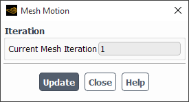
Important: The following options are not available for steady-state applications:
In-Cylinder
Implicit Update
Also, the Dynamic Mesh Events dialog box is not available for steady-state applications.
Consider a rescue drop case shown in Figure 13.94: Initial Object Position. The object can be moved in any position in the steady-state solver, after which steady-state analyses can be performed at different object positions.
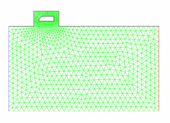
The dynamic mesh parameters setup is identical for the steady-state
and transient cases, which is described in Setting Dynamic Mesh Modeling Parameters. When setting up the dynamic
zones, the procedures are similar to those described in Specifying the Motion of Dynamic Zones, except that the UDF selected
from the Motion UDF/Profile drop-down list is
different. In steady-state cases the dtime passed to the UDF is by default 1. So, in this example, the object
will move 50 mm each time the following UDF is executed:
 #include "udf.h"

 DEFINE_CG_MOTION(pod,dt,vel,omega,time,dtime)

 {
  NV_S(vel,=,0);
  NV_S(omega,=,0);
  vel[1] = -50e-3;
 }
The resulting mesh is shown in Figure 13.96: Final Object Position After 40 Executions.