


Many problems involve multiple moving parts or contain stationary surfaces which are not surfaces of revolution (and therefore cannot be used with the Single Reference Frame modeling approach). For these problems, you must break up the model into multiple fluid/solid cell zones, with interface boundaries separating the zones. Zones that contain the moving components can then be solved using the moving reference frame equations (Equations for a Moving Reference Frame in the Theory Guide), whereas stationary zones can be solved with the stationary frame equations.
Multiple Reference Frame Model (MRF)
Sliding Mesh Model (SMM)
The MRF is a steady-state approximation whereas the SMM approach is inherently unsteady due to the motion of the mesh with time. This approach is discussed in Modeling Flows Using Sliding and Dynamic Meshes.
For additional information, see the following sections:
Additional information about the MRF model is presented in the following sections:
The MRF model [93] is, perhaps,
the simplest of the two approaches for multiple zones. It is a steady-state
approximation in which individual cell zones can be assigned different
rotational and/or translational speeds. The flow in each moving cell
zone is solved using the moving reference frame equations (see Introduction). If the zone is stationary ( ),
the equations reduce to their stationary forms. At the interfaces
between cell zones, a local reference frame transformation is performed
to enable flow variables in one zone to be used to calculate fluxes
at the boundary of the adjacent zone. For more information about the
MRF interface formulation, see The MRF Interface Formulation in the Theory Guide.
),
the equations reduce to their stationary forms. At the interfaces
between cell zones, a local reference frame transformation is performed
to enable flow variables in one zone to be used to calculate fluxes
at the boundary of the adjacent zone. For more information about the
MRF interface formulation, see The MRF Interface Formulation in the Theory Guide.
It should be noted that the MRF approach does not account for the relative motion of a moving zone with respect to adjacent zones (which may be moving or stationary); the mesh remains fixed for the computation. This is analogous to freezing the motion of the moving part in a specific position and observing the instantaneous flowfield with the rotor in that position. Hence, the MRF is often referred to as the “frozen rotor approach.”
While the MRF approach is clearly an approximation, it can provide a reasonable model of the flow for many applications. For example, the MRF model can be used for turbomachinery applications in which rotor-stator interaction is relatively weak, and the flow is relatively uncomplicated at the interface between the moving and stationary zones. In mixing tanks, for example, since the impeller-baffle interactions are relatively weak, large-scale transient effects are not present and the MRF model can be used.
Another potential use of the MRF model is to compute a flow field that can be used as an initial condition for a transient sliding mesh calculation. This eliminates the need for a startup calculation. The multiple reference frame model should not be used, however, if it is necessary to actually simulate the transients that may occur in strong rotor-stator interactions, the sliding mesh model alone should be used (see Modeling Flows Using Sliding and Dynamic Meshes.
For more information about and examples of multiple moving reference frames, see The Multiple Reference Frame Model in the Theory Guide.
The following limitations exist when using the MRF approach:
The interfaces separating a moving region from adjacent regions must be oriented such that the component of the frame velocity normal to the boundary is zero. This means that for a translationally moving frame, the moving zone’s boundaries must be parallel to the translational velocity vector. For rotating problems, the interfaces must be surfaces of revolution about the axis of rotation defined for the fluid zone. For the example shown Figure 2.4: Geometry with One Rotating Impeller (in the Theory Guide), this requires the dashed boundary to be circular (not square or any other shape).
Strictly speaking, the use of multiple reference frames is meaningful only for steady flow. However, Ansys Fluent will allow you to solve an unsteady flow when multiple reference frames are being used. In this case, unsteady terms (as described in Temporal Discretization in the Theory Guide) are added to all the governing transport equations. You should carefully consider whether this will yield meaningful results for your application, because, for unsteady flows, a sliding mesh calculation will generally yield more meaningful results than an MRF calculation.
By default, pathlines and particle trajectories drawn by Ansys Fluent use the velocity relative to the reference frame motion of the cell zone. However, for particle trajectories, you can change the reference frame by either selecting Track in Absolute Frame in the Numerics tab of the Discrete Phase Model dialog box or using the text command
define/models/dpm/options/track-in-absolute-frame.Note: When a pathline or particle trajectory crosses a boundary between zones with different reference frame motion specifications, you may observe a sharp change in particle velocity as a result of the coordinate transformation.
The particle injection velocities (specified in the Set Injection Properties Dialog Box) are interpreted in the same way as tracking, that is, either relative to the local frame of reference’s motion specification or in absolute coordinates.
You cannot accurately model axisymmetric swirl in the presence of multiple reference frames using the relative velocity formulation. This is because the current implementation does not apply the transformation used in Equation 2–16 (in the Theory Guide) to the swirl velocity derivatives. For this situation, the absolute velocity formulation should be used.
Translational and rotational velocities are assumed to be constant (time varying
 ,
,  are not allowed).
The relative velocity formulation cannot be used in combination with the MRF and mixture models. (For details, see Mixture Model Theory in the Theory Guide). For such cases, use the absolute velocity formulation instead.
You must not have a single interface between reference frames where part of the interface is made up of a coupled two-sided wall, while another part is not coupled (that is, the normal interface treatment). In such cases, you must break the interface up into two interfaces: one that is a coupled interface, and the other that is a standard fluid-fluid interface. See Using a Non-Conformal Mesh in Ansys Fluent for the steps involved in setting up a coupled interface.
Important: You can switch from the MRF model to the sliding mesh model for a more robust and
accurate solution, by using the
mesh/modify-zones/mrf-to-sliding-mesh text command. See Using Sliding Meshes for details on how to make this change in the
fluid’s boundary conditions.
Two mesh setup methods are available. Choose the method that is appropriate for your model, noting the restrictions in Limitations.
If the boundary between two zones that are in different reference frames is conformal (that is, the mesh node locations are identical at the boundary where the two zones meet), you can simply create the mesh as usual, with all cell zones contained in the same mesh file. A different cell zone should exist for each portion of the domain that is modeled in a different reference frame. Use an interior zone for the boundary between reference frames.
If the boundary between two zones that are in different reference frames is non-conformal (that is, the mesh node locations are not identical at the boundary where the two zones meet), follow the non-conformal mesh setup procedure described in Using a Non-Conformal Mesh in Ansys Fluent.
To learn more about setting up a multiple reference frame problem, see the following sections:
To model a problem involving multiple reference frames, perform the following:
Important: The mesh-setup constraints for a moving reference frame listed in Mesh Setup for a Single Moving Reference Frame apply to multiple reference frames as well.
Select the Velocity Formulation to be used in the General Task Page: either Absolute or Relative. (For details, see Choosing the Relative or Absolute Velocity Formulation.)
 Setup →
  General
(Note that this step is irrelevant if you are using one of the density-based solution algorithms; these algorithms always use an absolute velocity formulation.)
For each cell zone in the domain, specify its translational velocity and/or its angular velocity (
 ) and the axis about which it rotates. Setup → Cell Zone
Conditions
) and the axis about which it rotates. Setup → Cell Zone
Conditions
If the zone is moving, or if you plan to specify cylindrical velocity or flow-direction components at inlets to the zone, you must define the axis of rotation of the frame of reference. In the Fluid or Solid dialog box, specify the Rotation-Axis Origin and Rotation-Axis Direction under the Reference Frame tab.
In the Fluid (Figure 10.4: The Fluid Dialog Box Displaying Frame Motion Inputs) or Solid dialog box, enable the Frame Motion option. (Note that a solid zone cannot move at a different speed than an adjacent solid zone; for such a situation, you must instead use Solid Motion.)
In the Reference Frame tab, set the Speed under Rotational Velocity and/or the X, Y, and Z components of the Translational Velocity. Note that the speed can be specified as a constant value or a transient profile. The transient profile may be in a file format, as described in Transient Cell Zone and Boundary Conditions, or a UDF macro, described in
DEFINE_TRANSIENT_PROFILE. Specifying the individual velocities as either a profile or a UDF allows you to specify a specific input of the frame motion individually. However, you can also specify the frame motion inputs via a single user-defined function that uses the UDF macroDEFINE_ZONE_MOTION. This may prove to be quite convenient if you are modeling a more complicated motion of the moving reference frame, where the hooking of many different user-defined functions or profiles can be cumbersome.Note: If you decide to hook a UDF, then you will no longer have access to the rotation axis origin and direction, or the velocities.
Details about these inputs are presented in Inputs for Fluid Zones and in Inputs for Solid Zones. Details about the zone motion UDF can be found in
DEFINE_ZONE_MOTIONin the Fluent Customization Manual.To switch between the MRF and moving mesh models, click the Copy To Mesh Motion for zones with a moving frame of reference and Copy to Frame Motion for zones with moving meshes to transfer motion variables, such as the axes, frame origin, and velocity components between the two models.
The variables used for the origin, axis, and velocity components, as well as for the UDF
DEFINE_ZONE_MOTIONwill be copied. This is particularly useful if you are doing a steady-state MRF simulation to obtain an initial solution for a transient Moving Mesh simulation in a turbomachine.
Define the velocity boundary conditions at walls. You can choose to define either an absolute velocity or a velocity relative to the velocity of the adjacent cell zone specified in step 2.
If the wall is moving at the speed of the moving frame (and hence stationary relative to the moving frame), it is convenient to specify a relative angular velocity of zero. Likewise, a wall that is stationary in the non-moving frame of reference should be given a velocity of zero in the absolute reference frame. Specifying the wall velocities in this manner obviates the need to modify these inputs later if a change is made in the rotational velocity of the fluid zone.
An example for which you would specify a relative velocity is as follows: If an impeller is defined as wall-3 and the fluid region within the impeller’s radius is defined as fluid-5, you would need to specify the angular velocity and axis of rotation for fluid-5 and then assign wall-3 a relative velocity of 0. If you later wanted to model a different angular velocity for the impeller, you would need to change only the angular velocity of the fluid region; you would not need to modify the wall velocity conditions.
Details about these inputs are presented in Velocity Conditions for Moving Walls.
Define the boundary conditions at the inlets, as described in Boundary Conditions. For velocity inlets, you can choose to define either absolute velocities or velocities relative to the motion of the adjacent cell zone (specified in step 2). Likewise, the total pressure and flow direction can be prescribed in absolute or relative frames for pressure inlets.
Details about these inputs are presented in Defining the Flow Direction and Defining the Velocity.
Define the mesh interfaces using the Mesh Interfaces Dialog Box (Figure 13.10: The Mesh Interfaces Dialog Box).
Setup → Mesh
Interfaces New...
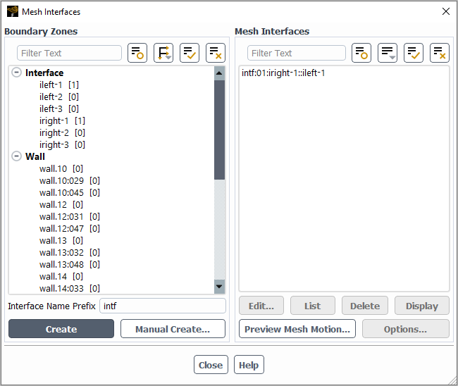
To learn how to use the Mesh Interfaces dialog box, see Using a Non-Conformal Mesh in Ansys Fluent.
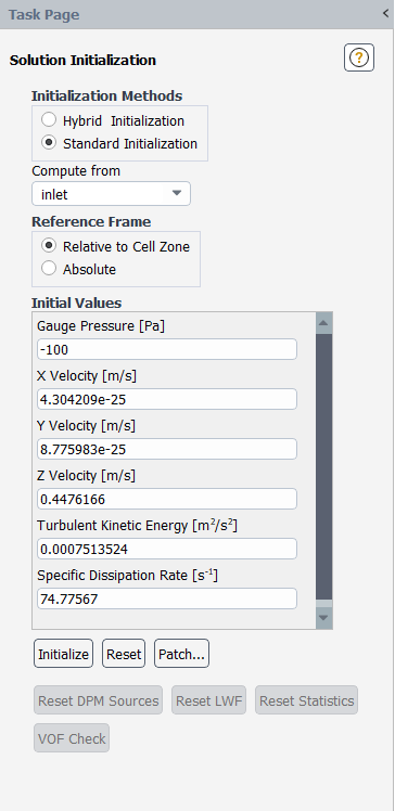
Initialize the solution using an absolute frame of reference (Figure 10.8: The Solution Initialization Task Page for Moving Reference Frames).
Solution →
Initialization
Select the Absolute option under Reference Frame. If the Relative to Cell Zone option is selected, the initial flow field can contain discontinuities, which can cause convergence problems in the first few iterations.
(optional) For transient cases, after you have initialized or run the calculation you can use the Moving Mesh Courant Number field variable (in the Velocity... category) to guide your solution. This field variable is a non-dimensional value that indicates the number of cells that might be swept in a single time step due to a mesh motion.
For multiple moving reference frames, follow the guidelines presented in Solution Strategies for a Single Moving Reference Frame for a single moving reference frame. Remember that with multiple zones, the possibility exists of interaction between moving and stationary components. This will manifest itself as poor or oscillatory convergence. In such cases, it is strongly recommend that the sliding mesh approach be used to compute the flowfield in order to resolve the unsteady interactions.
When you solve a problem using the multiple reference frame model, you can plot or report both absolute and relative velocities. For all velocity parameters (for example, Velocity Magnitude and Mach Number), corresponding relative values will be available for postprocessing (for example, Relative Velocity Magnitude and Relative Mach Number). These variables are contained in the Velocity... category of the variable selection drop-down list that appears in postprocessing dialog boxes. Relative values are also available for postprocessing of total pressure, total temperature, and any other parameters that include a dynamic contribution dependent on the reference frame (for example, Relative Total Pressure, Relative Total Temperature).
Important: Relative velocities are relative to the translational/rotational velocity of the “reference zone” (specified in the Reference Values task page (see Reference Values Task Page)). The velocity of the reference zone is the velocity defined in the Fluid Dialog Box for that zone.
When plotting velocity vectors, you can choose to plot vectors in the absolute frame (the default), or you can select Relative Velocity in the Vectors of drop-down list in the Vectors Dialog Box to plot vectors relative to the translational/rotational velocity of the “reference zone” (specified in the Reference Values Task Page). If you plot relative velocity vectors, you might want to color the vectors by relative velocity magnitude (by choosing Relative Velocity Magnitude in the Color by list); by default they will be colored by absolute velocity magnitude.
You can also generate a plot of circumferential averages in Ansys Fluent. This allows you to find the average value of a quantity at several different radial or axial positions in your model. Ansys Fluent computes the average of the quantity over a specified circumferential area, and then plots the average against the radial or axial coordinate. For more information on generating XY plots of circumferential averages, see XY Plots of Circumferential Averages.
For details about turbomachinery-specific postprocessing features, see Turbomachinery Postprocessing.