


After you have completed your discrete phase inputs and any coupled two-phase calculations of interest, you can display and store the particle trajectory predictions. Ansys Fluent provides both graphical and alphanumeric reporting facilities for the discrete phase, including the following:
graphical display of the particle trajectories
summary reports of trajectory fates
step-by-step reports of the particle position, velocity, temperature, and diameter
alphanumeric reports and graphical display of the interphase exchange of momentum, heat, and mass
optionally, alphanumeric reports and graphical display of various cell-averaged discrete phase field variables
sampling of trajectories at boundaries and lines/planes
summary reporting of current particles in the domain
histograms of trajectory data at sample planes
display of erosion/accretion rates
exporting of trajectories to Fieldview and Ensight
This section provides detailed descriptions of each of these postprocessing options.
(Note that plotting or reporting trajectories does not change the source terms.)
For additional information, see the following sections:
- 24.9.1. Displaying of Trajectories
- 24.9.2. Particle Tracking Statistics
- 24.9.3. Summary Reports
- 24.9.4. Step-by-Step Reporting of Trajectories
- 24.9.5. Reporting of Current Positions for Unsteady Tracking
- 24.9.6. Reporting of Interphase Exchange Terms (Discrete Phase Sources)
- 24.9.7. Reporting of Particle Variables
- 24.9.8. Reporting of Discrete Phase Variables
- 24.9.9. Reporting of Unsteady DPM Statistics
- 24.9.10. Sampling of Trajectories
- 24.9.11. Histogram Reporting of Samples
- 24.9.12. Contour Plots of DPM Particle Sampling Results on a Planar Surface
- 24.9.13. Summary Reporting of Current Particles
- 24.9.14. Postprocessing of Erosion/Accretion Rates
- 24.9.15. Assessing the Risk for Solids Deposit Formation During Selective Catalytic Reduction Process
When you have defined discrete phase particle injections, as described in Setting Initial Conditions for the Discrete Phase, you can display the trajectories of these discrete particles using the Particle Tracks Dialog Box (Figure 24.59: The Particle Tracks Dialog Box).
You can create named particle track definitions and save them for later use. See Creating and Using Contour Plot Definitions for additional information on graphics object definitions.
Note that particle track definitions can be included in scenes as long as the XY Plot option is not enabled. See Displaying a Scene for additional information on scenes.
![]() Results → Graphics →
Particle Tracks
Results → Graphics →
Particle Tracks ![]() Edit...
Edit...
You can also create a named particle track plot definition and save it for later use.
![]() Results → Graphics →
Particle Tracks
Results → Graphics →
Particle Tracks ![]() New...
New...
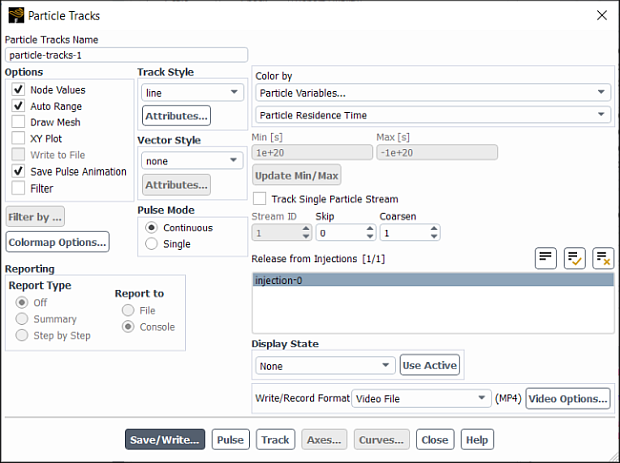
The procedure for drawing trajectories for particle injections is as follows:
Select the particle injection(s) you want to track in the Release from Injections list. (You can choose to track a specific particle, instead, as described below.)
If you have not done this yet, set the Step Length Factor and the Max. Number of Steps (Tracking tab) in the Discrete Phase Model Dialog Box.
 Setup → Models → Discrete Phase
  Edit...
If stochastic tracking is desired, set the related parameters in the Set Injection Properties dialog box, as described in Stochastic Tracking.
Note: Displaying tracks multiple times at the same solution state will result in identical random tracks. This is because the same seeding is used enabling you to postprocess different variables on the same particle tracks.
(optional) Specify which particles you want to display.
If you want to display a single particle stream, enable Track Single Particle Stream and specify the particle stream ID number in the Stream ID field.
Note:To determine the stream ID in the injection of interest, use the Injections Dialog Box to list the injection particle streams, as described in Listing Injection Initial Conditions. The stream ID numbers will be listed in the first column of the data printed in the Ansys Fluent console.
For unsteady tracking, all of the particles related to the specified injection stream will be displayed. The displayed data will not correspond to the time history of an individual particle.
(wall film model only) Enable Free Stream Particles and/or Wall Film Particles if you want to display those types of particles. Note that these options are available only when the Lagrangian wall film model is enabled in the wall boundary conditions dialog box, under the DPM tab.
Set any of the display options described below.
Click the (or Save/Display) button to draw the trajectories or click the button to animate the particle positions. The button will become the button during the animation, and you must click to stop the pulsing.
Note: Enable Save Pulse Animation to save a video or picture files of the pulse animation. When this option is enabled, an additional Write/Record Format drop-down list appears that controls what type of file is written when you click Save/Write....
A Continuous pulse video file will be 5 seconds long, while a Single pulse video will be one full cycle.
Important:For unsteady particle tracking simulations, clicking will show only the current location of the particles. Typically, you should select point in the Track Style drop-down list when displaying transient particle locations since individual positions will be displayed.
The button option is not available for unsteady tracking.
(Optional) Associate a display state with this particle tracks plot for a consistent appearance each time the particle tracks are redisplayed.
Set the display state. There are two approaches:
Setup the graphics window with your preferred model orientation, zoom level, graphics effects, ruler, and so on, and click to create a display state with these properties.
Select a display state from the Display State drop-down list (if you already created a display state that you would like to reuse for other graphics objects).
Click to link the selected display state with this particle tracks plot.
Refer to Controlling the Display State and Modifying the View for additional information.
Note: If you experience an uncharacteristic delay in the displaying of particle tracks (with Track Style set to line and/or Vector Style set to vector), disabling the Hover-Over Probe Values option in Preferences (located in the Appearance branch under Selections) should restore the display performance.
You can include the mesh in the trajectory display, control the style of the trajectories (including the twisting of ribbon-style trajectories), color them by different scalar fields and control the color scale, and coarsen trajectory plots. (More information about these options can be found in Controlling the Particle Tracking Style and Controlling the Vector Style of Particle Tracks.) You can also choose node or cell values for display. If you are “pulsing” the trajectories, you can control the pulse mode and save an animation of the pulse. Finally, you can generate an XY plot of the particle trajectory data (for example, residence time) as a function of time or path length and save this XY plot data to a file.
Note: The Draw Mesh option settings are not saved with the particle track plot definition. Once the dialog box is closed these settings will revert to being disabled. If you want these settings persisted within the current session, you can use the non-persistent Particle Tracks dialog box.
![]() Results → Graphics
→
Particle Tracks
→
New...
Results → Graphics
→
Particle Tracks
→
New...
Plotting particle trajectories can be very time consuming, therefore,
to reduce the plotting time, a coarsening factor can be used to reduce
the number of points that are plotted. Providing a coarsening factor
of  , will result in each
  th point
being plotted for a given trajectory in any cell. This coarsening
factor is specified in the Particle Tracks Dialog Box, in the Coarsen field and is only valid for
steady-state cases. For example, if the coarsening factor is set to
2, then Ansys Fluent will plot alternate points.
th point
being plotted for a given trajectory in any cell. This coarsening
factor is specified in the Particle Tracks Dialog Box, in the Coarsen field and is only valid for
steady-state cases. For example, if the coarsening factor is set to
2, then Ansys Fluent will plot alternate points.
Important: Note that if any particle or pathline enters a new cell, this point will always be plotted.
To reduce plotting time in transient cases, Ansys Fluent has available
an option to skip plotting every  particle
in an injection. Selecting this option is also done in the Particle Tracks Dialog Box by specifying a nonzero integer
in the Skip field. For example, if an individual
stream is selected and the skip option is set to 1, every other particle
will be plotted. If the entire injection is selected with a skip option
of 1, every other particle will be plotted for all streams in the
injection.
particle
in an injection. Selecting this option is also done in the Particle Tracks Dialog Box by specifying a nonzero integer
in the Skip field. For example, if an individual
stream is selected and the skip option is set to 1, every other particle
will be plotted. If the entire injection is selected with a skip option
of 1, every other particle will be plotted for all streams in the
injection.
These options are controlled in exactly the same way that pathline-plotting options are controlled. See Options for Pathline Plots for details about setting the trajectory plotting options mentioned above.
Note that in addition to coloring the trajectories by continuous phase variables, you can also color them according to the discrete phase variables summarized in Reporting of Particle Variables. To display the minimum and maximum values in the domain, click the button.
Particle tracking can be displayed as lines (with or without arrows), ribbons, cylinders (coarse, medium, or fine), triangles, spheres, refined spheres, or a set of points. In the Track Style drop-down list in the Particle Tracks dialog box, you can choose:
(steady tracking) line, line-arrows, point, sphere, refined-sphere, ribbon, triangle, coarse-cylinder, medium-cylinder, or fine-cylinder.
(unsteady tracking) point, sphere, or refined-sphere.
Important:
The main difference between the sphere, and the refined-sphere option is that the refined-sphere is a higher quality sphere that has better performance (frames per second). The performance decreases when the diameter of the sphere is too large (for example, 10 or more).
Reflections and shadows are not shown for the style.
Pulsing can be done only on point, sphere, refined-sphere, or line styles.
Once you have selected the track style, click the button to specify how you would like to display the particle tracks.
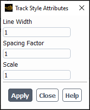
If you are using the line or line-arrows style, set the Line Width in the Track Style Attributes dialog box (Figure 24.60: The Track Style Attributes Dialog Box) that appears when you click the button. For line-arrows you will also set the Spacing Factor, which controls the spacing between the particles tracks. The size of the arrow heads can be adjusted by entering a value in the Scale text-entry box.
If you are using the point style, you will set the Marker Size in the Track Style Attributes dialog box. The thickness of the particle track will be the thickness of the marker.
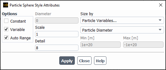
If you are using the sphere style, you will set the Diameter, scale, and Detail in the Particle Sphere Style Attributes dialog box (Figure 24.61: The Particle Sphere Style Attributes Dialog Box). You have the option of specifying a constant diameter if you enable Constant under Options and you will then specify the Diameter. If you enable Variable, you can select a particle variable to estimate the size of the spheres. The spheres are scaled by the factor entered in the Scale entry box.
The best constant diameter to use will depend on the dimensions of the domain, the view, and the particle density. However, an adequate starting point would be a diameter on the order of 1/4 of the average cell size or 1/4 step size. Units for the Diameter field correspond to the mesh dimensional units.
The level of detail applied to the graphical rendering of the spheres can be controlled using the Detail field. The level of detail uses integer values ranging from 4 to 50. Note that the performance of the graphical rendering as well as the memory consumption will be better when using a small level of detail, that is, very coarse spheres, such as 6 or 8. The rendering performance significantly decreases with higher levels of detail. You should gradually increase the detail to determine the best-case scenario between performance and quality.
Whenever Auto Range is disabled, the spheres are displayed only if they have values between Min and Max.
Also note that to take full advantage of spherical rendering, lighting should be turned on in the view. The Gouraud setting provides much smoother looking spheres than the Flat setting and better performance than the Phong setting. For more information on lighting, see Adding Lights.
If you are using the refined-sphere, you can set the Diameter and the Scale in Figure 24.61: The Particle Sphere Style Attributes Dialog Box.
If you are using the triangle or any of the cylinder styles, you will set the Width in the Track Style Attributes dialog box. For triangles, the specified value will be half the width of the triangle’s base, and for cylinders, the value will be the cylinder’s radius.
If you are using the ribbon style, clicking on the button will open the Ribbon Attributes Dialog Box, in which you can set the ribbon’s Width. You can also specify parameters for twisting the ribbon tracks. In the Twist By drop-down list, you can select a scalar field on which the tracks twisting is based (for example, helicity). Select the desired category in the upper list and then select a related quantity in the lower list. The twisting may not be displayed smoothly because the scalar field by which you are twisting the tracks is calculated at cell centers only (and not interpolated to a particle’s position). The Twist Scale sets the amount of twist for the selected scalar field. To magnify the twist for a field with very little change, increase this factor; to display less twist for a field with dramatic changes, decrease this factor.
When you click , the Min and Max fields will be updated to show the range of the Twist By scalar field.
You can choose to have the particle tracks displayed as vectors. Choose the Vector Style from the drop-down list in the Particle Tracks dialog box:
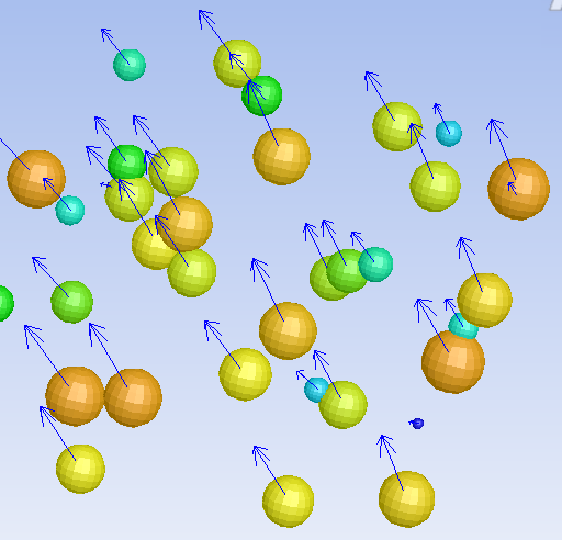
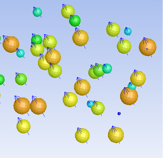
If you select vector, the vector will be generated starting in the center of the particle, as shown in Figure 24.62: Particles with the Vector Style.
If you select centered-vector, the midpoint of the vector will appear in the center of the particle, as shown in Figure 24.63: Particles with the Centered Vector Style.
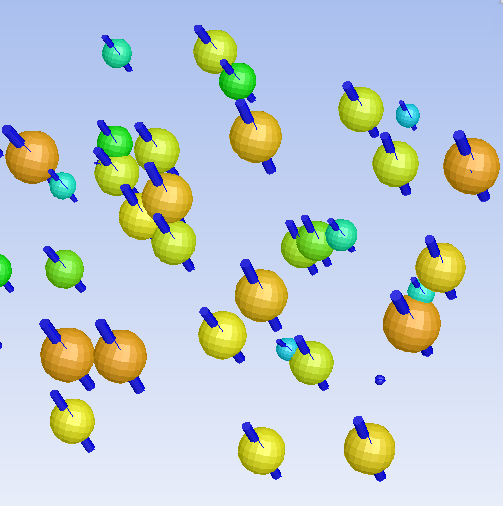
If you select centered-cylinder, the midpoint of the cylinder will appear in the center of the particle, as shown in Figure 24.64: Particles with the Centered Cylinder Style.
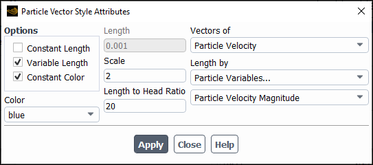
Click the button to specify how you would like to display the particle tracks. In the Particle Vector Style Attributes dialog box (Figure 24.65: The Particle Vector Style Attributes Dialog Box) you will set the Length, Scale, and Length to Head Ratio. The direction of the vectors is displayed for the selected variable under Vectors of. You have the option of specifying a Constant Length or a Variable Length, which is based on the variable selected under Length by. If Constant Color is enabled, then all vectors/cylinders are colored by the color selected in the Color drop-down list. Otherwise, it is the color selected in the Particle Tracks dialog box (seen in the Mesh Colors dialog box when Draw Mesh is enabled).
Vectors can be scaled by the factor given in the Scale entry box. The ratio of vector length to vector head size can be changed in the box Length to Head Ratio. In the case of a cylinder, the ratio of the length to the diameter is affected.
For transient simulations, you can use the Import Particle Data dialog box (Figure 24.66: The Import Particle Data Dialog Box) to import particle data to display in the graphics window.
![]() Results → Model Specific
→ Discrete Phase → Import Particle
Data...
Results → Model Specific
→ Discrete Phase → Import Particle
Data...
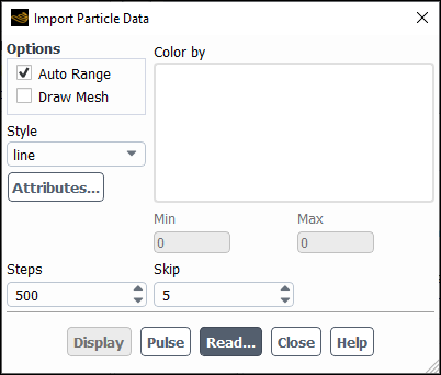
Click to display a file selection dialog box where you can enter a file name and a directory that contains the imported data.
Choose from the available import options by selecting Auto Range and/or Draw Mesh under Options. If you prefer to restrict the range of the scalar field, disable the Auto Range option and set the Min and Max values manually beneath the Color by list.
Choose to color the particle pathlines by any of the scalar fields in the Color by list. If you select COLORBY, the pathlines will be colored by the quantity that was chosen when the particle data file was created. (See Exporting Steady-State Particle History Data)
Select a pathline style under Style. To set pathline style attributes, click the button. For more information about the pathline style types, see Controlling the Pathline Style.
The value of Steps sets the maximum number of steps a particle can advance. A particle will stop when it has traveled this number of steps or when it leaves the domain.
If your pathline plot is difficult to understand because there are too many paths displayed, you can “thin out” the pathlines by changing the Skip value.
Click the button to draw the pathlines, or click the button to animate the particle positions. The button will become the button during the animation, and you must click to stop the pulsing.
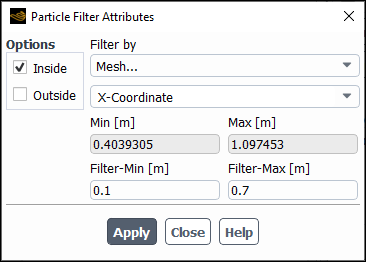
You can specify how you would like to filter the particles being displayed, by first enabling the Filter option in the Options group of the Particle Tracks dialog box, then clicking the button. In the Particle Filter Attributes dialog box, select the field variable by which you want to filter, then specify whether you would like to display all the particle tracks Inside or Outside the Filter-Min and Filter-Max range, as shown in Figure 24.67: The Particle Filter Attributes Dialog Box.
Note: All particle variables as well as any field variable except for Custom Field Functions... can be used as a filter variable.
For axisymmetric problems in which the particle has a nonzero
circumferential velocity component, the trajectory of an individual
particle is often a spiral about the centerline of rotation. Ansys Fluent displays
the  and
and  components of the trajectory (but not the
  component) projected
in the axisymmetric plane.
component) projected
in the axisymmetric plane.
During two-way coupled DPM calculations or when you do graphical postprocessing of steady particle trajectories (as described in Displaying of Trajectories), Ansys Fluent prints tracking statistics in the console. For example:
 DPM Iteration ....
  number tracked = 7, escaped = 4, aborted = 0, trapped = 0, evaporated = 3
 Done.
The above numbers report events that the numerical parcels may have undergone. They should not be taken for any physically meaningful information since numerical parcels may represent different amounts (particle counts) of the particulate phase.
The description of particle statuses can be found in Trajectory Fates.
By default, only those events that have occurred at least once are reported. This can be
changed using the define/models/dpm/numerics/tracking-statistics text
command.
You can also track particles through the domain without displaying the trajectories by clicking the button at the bottom of the Particle Tracks dialog box. This allows the listing of reports without also displaying the tracks.
You can request additional detail about the trajectory fates as the particles exit the domain, including the mass flow rates through each boundary zone, mass flow rate of evaporated droplets, and composition of the particles.
Follow steps 1 and 2 in Displaying of Trajectories for displaying trajectories.
Select Summary as the Report Type and click or .
Important: For steady-state simulations, DPM summary data is not stored in the
.datfile, since it is possible to track particles on single or combinations of injections. Transient simulations store this data since it is accumulated over time starting from initialization.
A detailed report similar to the following example will appear in the console window. (You may also choose to write this report to a file by selecting File as the Report to option, clicking the button (which was originally the Display button), and specifying a file name for the summary report file in The Select File Dialog Box.)
 number  tracked  =  10,  escaped  =  3,  aborted  =  0,  trapped  =  5,  evaporated  =  2,

 Fate          Zone Zone Number                  Elapsed Time (s)     Injection, Index Injection, Index
               Name   Id             Min       Max       Avg   Std Dev             Min              Max
 ---------- ------- ---- ----- --------- --------- --------- --------- ----------- --- ----------- ----
 Evaporated                  2 1.770e-03 1.114e-02 6.456e-03 4.686e-03 injection-0   2 injection-0   76
 Escaped    outflow    6     3 6.043e-01 7.037e-01 6.471e-01 4.172e-02 injection-1   4 injection-1   72
 Trapped       wall    7     5 8.486e-03 1.767e-01 5.030e-02 6.421e-02 injection-1   8 injection-1   75

                                  (*)- Mass Transfer Summary -(*)

 Fate           Zone   Zone       Mass Flow (kg/s)
                Name     Id    Initial      Final     Change
 ----------- ------- ------ ---------- ---------- ----------
 Evaporated                  8.333e-02  0.000e+00 -8.333e-02
 Escaped     outflow      6  1.167e-01  5.144e-02 -6.523e-02
 Trapped        wall      7  2.000e-01  2.400e-02 -1.760e-01
 -----------                ---------- ---------- ----------
 Net                         4.000e-01  7.544e-02 -3.246e-01

                                  (*)- Energy Transfer Summary -(*)

 Fate           Zone   Zone      Heat Rate (W)          Change of Heat (W)
                Name     Id    Initial      Final   Sensible     Latent      Total
 ----------- ------- ------ ---------- ---------- ---------- ---------- ----------
 Evaporated                 -3.180e+04  0.000e+00 -3.382e+02  3.214e+04      1.107
 Escaped     outflow      6  5.272e+05  6.519e+05 -3.487e+03  1.282e+05      1.523
 Trapped        wall      7  4.954e+05  6.993e+05 -1.173e+03  2.051e+05      1.737
 -----------                ---------- ---------- ---------- ---------- ----------
 Net                         9.908e+05  1.351e+06 -4.998e+03  3.654e+05      4.367

                                  (*)- Combusting Particles -(*)

 Fate           Zone   Zone   Volatile Content (kg/s)        Char Content (kg/s)
                Name     Id    Initial      Final   %Conv    Initial      Final   %Conv
 ----------- ------- ------ ---------- ---------- ------- ---------- ---------- -------
 Evaporated                  0.000e+00  0.000e+00    0.00  0.000e+00  0.000e+00     100
 Escaped     outflow      6  9.333e-03  9.333e-03    0.00  2.133e-02  2.133e-02       0
 Trapped        wall      7  9.333e-03  7.485e-01  100.00  2.133e-02  2.133e-02      98
 -----------                ---------- ---------- ------- ---------- ---------- -------
 Net                         1.867e-02  9.333e-03  50.00  4.267e-02  4.267e-02      198

                                  (*)- Multicomponent Droplet -(*)

 Fate           Zone   Zone               Species      Species Content (kg/s)
                Name     Id                 Names    Initial      Final   %Conv
 ----------- ------- ------ --------------------- ---------- ---------- -------
 Evaporated                      c5h12-droplet<l>  1.667e-02  0.000e+00  100.00
 Evaporated                      c7h16-droplet<l>  3.333e-02  0.000e+00  100.00
 Evaporated                                h2o<l>  0.000e+00  0.000e+00    0.00
 Escaped    outflow       6      c5h12-droplet<l>  1.667e-02  2.585e-04   98.45
 Escaped    outflow       6      c7h16-droplet<l>  0.000e+00  0.000e+00    0.00
 Escaped    outflow       6                h2o<l>  3.333e-02  1.134e-02   65.99
 Trapped       wall       7      c5h12-droplet<l>  3.333e-02  0.000e+00  100.00
 Trapped       wall       7      c7h16-droplet<l>  3.333e-02  0.000e+00  100.00
 Trapped       wall       7                h2o<l>  3.333e-02  0.000e+00  100.00
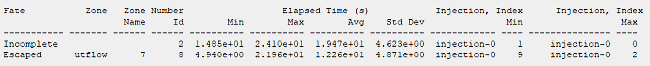
The report groups together particles with each possible fate, and reports the number of particles, the time elapsed during trajectories, and the mass and energy transfer This information can be very useful for obtaining information such as where particles are escaping from the domain, where particles are colliding with surfaces, and the extent of heat and mass transfer to/from the particles within the domain. Additional information is reported for combusting particles and multicomponent particles.
For cases with multiple injections, note the following:
If you select only one injection from the Release from Injections list in the Sample Trajectories dialog box, available information is reported for that injection. There may not be any information available for individual flow boundaries unless you issued the text command
/report/dpm-zone-summaries-per-injection?prior to the particle tracking.If you select more than one injection, Fluent produces the DPM summary report for all injections, even if only a subset was selected from the Release from Injections list.
Note that for cases with unsteady particle tracking, information about particle parcels still residing within the computational domain is only reported if you use the Display button (not the Track button). If you require this information but are not interested in the graphical display, you can use the Display button but set the Skip entry to a very large number and make sure Draw Mesh is cleared.
For details, see the following sections:
- 24.9.3.1. Trajectory Fates
- 24.9.3.2. Elapsed Time
- 24.9.3.3. Mass Transfer Summary
- 24.9.3.4. Energy Transfer Summary
- 24.9.3.5. Heat Rate and Energy Reporting
- 24.9.3.6. Combusting Particles
- 24.9.3.7. Combusting Particles with the Multiple Surface Reaction Model
- 24.9.3.8. Multicomponent Particles
- 24.9.3.9. Reinjected Particles
- 24.9.3.10. Evaporated Mass
The possible fates for a particle trajectory are as follows:
“Escaped” trajectories are those that terminate at a flow boundary for which the “escape” condition is set.
“Incomplete” trajectories are those that were terminated when the maximum allowed number of time steps — as defined by the Max. Number of Steps input in the Discrete Phase Model Dialog Box (see Numerics of the Discrete Phase Model) — was exceeded.
“Incomplete_parallel” may appear as an additional fate for parallel simulations. This means that the number of particle exchanges between partitions has been exceeded. Any remaining particles on the compute nodes are stopped, which is indicated by the number following this fate. Therefore no further source terms from these particles are considered. The number of particle exchanges is limited to avoid very long computational time due to incomplete particles. You can change the default value of 1000 to a value of 20000 with a scheme command. Contact the technical support engineer for this information.
“Trapped” trajectories are those that terminate at a flow boundary where the “trap” condition has been set.
“Evaporated” trajectories include those trajectories along which the particles were evaporated within the domain.
“Aborted” trajectories are particles that have become trapped at interior faces (DPM particles) or edges (Lagrangian wall-film particles) due to discontinuities in the forces on the particle. Make sure you enable interpolation for the flow density, viscosity, wall-film properties, and so on. This may reduce the number of aborted particles if these properties vary spatially.
“Shed” trajectories are newly generated particles during the breakup of a larger droplet. They appear only if a breakup model is enabled.
“Coalesced” trajectories are removed particles which have coalesced after particle-particle collisions. They appear only if the coalescence model is enabled.
“Splashed” trajectories are particles that are newly generated when a particle touches a wall film. Those trajectories appear only if the wall film model is enabled.
(DPM summary reports only) “Injected” trajectories are sums over all particles injected.
If Unsteady Particle Tracking is enabled, the following additional fates may be reported:
"Transformed" are particle parcels that have been replaced by other parcels (compare with the "Inserted" fate below) or by a representation of the same amount of fluid in the Eulerian formulation.
"Inserted" are particle parcels that have been added to the simulation by any way other than from an injection. These can include secondary break-up, condensation, any kind of film interaction and model transition between, for example, Eulerian VOF and DPM.
"In Fluid" particle parcels are free-stream particle parcels that are still travelling in the domain at the current point in time and have not reached any final destiny yet.
"In Film" particle parcels are Lagrangian wall-film particle parcels that are still inside the computational domain at the current point in time and have not reached any final destiny yet.
"filmrelease" particle parcels are Lagrangian wall-film particle parcels that are released into the free stream but not assigned a particle diameter based on a physical model (such as stripping or separation). If many such events are reported, you may need to improve the case setup for best possible predictions. This fate may appear in the tracking statistics (see Particle Tracking Statistics).
In DPM summary reports, "Escaped" and "Trapped" fates are reported separately for every
flow boundary. Note that this is not true if there are multiple injections in the case, and the
DPM summary report is produced for a single injection (as opposed to a single report for all
injections). To record trajectory fates per individual flow boundary for every injection
separately, you can use the text command
/report/dpm-zone-summaries-per-injection? prior to the particle
tracking. In a case with unsteady particle tracking, you need to issue this command before the
first particle is injected. All other fates are always recorded for every injection separately.
The number of particles with each fate is listed under the Number
heading. (Particles that escape through different zones or are trapped at different zones are
considered to have different fates, and are therefore listed separately.) The minimum, maximum,
and average time elapsed during the trajectories of these particles, as well as the standard
deviation about the average time, are listed in the Min,
Max, Avg, and Std
Dev columns. This information indicates how much time the particle(s) spent in
the domain before they escaped, aborted, evaporated, or were trapped. Also, on the right side
of the report, the injection name and index of the trajectories with the minimum and maximum
elapsed times. (You may need to use the scroll bar to view this information.)
For all droplet or combusting particles with each fate, the total initial and final mass
flow rates and the change in mass flow rate are reported in the
Initial, Final, and
Change columns. With this information, you can determine how much
mass was transferred to the continuous phase from the particles.
For unsteady tracking, the report lists the time-integrated mass flow rate of the particle streams that have reached a particular fate at the current flow time. In other words, the report does not include particles that are still being tracked in the domain.
                           (*)- Mass Transfer Summary -(*)

 Fate              Zone   Zone       Mass Flow (kg/s)
                   Name     Id    Initial      Final     Change
 ----------- ---------- ------ ---------- ---------- ----------
 Incomplete                     1.388e-03  1.943e-04  1.194e-03
Escaped outflow 7 1.683e-01 7.124e-02 -9.709e-02This report tells you how much heat was transferred from the particles to the continuous
phase. The report is organized in two sections. For steady simulations, there is a
Heat Rate and a Change of Heat section. For
unsteady particle tracking, there is an Energy and a
Change of Energy section. The Heat Rate and
Energy sections are the same for all particle types, while the other
sections report the change of heat due to the various transfer processes, which differ for each
particle type. For steady simulations, the report lists the rate and the change of heat for the
particle streams organized according to the particle stream fates. For unsteady tracking, the
report lists the time integrated heat rate and change of the particle streams that have reached
a particular fate at the current flow time. Note that the report does not include particles
that are still being tracked in the domain.
For all particles with each fate, the total initial and final heat content are reported in
the Initial and Final columns. The particle
heat content  is defined as follows:
Inert Particles:
 | (24–15) |
| where: | |
 = mass flow rate of particles (kg/s) = mass flow rate of particles (kg/s) | |
 = temperature of particles (K) = temperature of particles (K) | |
 = heat capacity of particles (J/kg/K) = heat capacity of particles (J/kg/K) | |
 = reference temperature for enthalpy (K) = reference temperature for enthalpy (K) |
Droplet Particles:
 | (24–16) |
| where: | |
 = heat of pyrolysis (J/kg) = heat of pyrolysis (J/kg) | |
 = latent heat of evaporation at reference conditions (J/kg) = latent heat of evaporation at reference conditions (J/kg) |
The latent heat at the reference conditions  is defined in Equation 12–509 in
the Theory Guide.
is defined in Equation 12–509 in
the Theory Guide.
Combusting Particles:
 | (24–17) |
 is the heat content of the evaporating/boiling liquid material if Wet
Combustion is selected (otherwise
is the heat content of the evaporating/boiling liquid material if Wet
Combustion is selected (otherwise  = 0).
= 0).
 | (24–18) |
| where: | |
 is the mass fraction of the liquid in the combusting particle is the mass fraction of the liquid in the combusting particle | |
 , ,  , and , and  are properties of the evaporating liquid material are properties of the evaporating liquid material |
 is the heat content of the dry combusting particle and is calculated as
 | (24–19) |
| where: | |
 is the volatile fraction is the volatile fraction | |
 is the combustible fraction is the combustible fraction |
Important: The Heat Rate section of the report is not provided for the
multiple surface reactions model.
Multicomponent Particles:
 | (24–20) |
| where: | |
 = mass fraction of component i in particle = mass fraction of component i in particle | |
 = heat content of component i = heat content of component i |
and
 | (24–21) |
| where: | |
 = heat of pyrolysis for component i (J/kg) = heat of pyrolysis for component i (J/kg) | |
 = latent heat of evaporation at reference conditions for component i
(J/kg) = latent heat of evaporation at reference conditions for component i
(J/kg) | |
 = specific heat of component i (J/kg/K) = specific heat of component i (J/kg/K) |
This section reports the total heat transferred from the particle to the continuous phase
and is analyzed in components of Sensible heat,
Latent heat and heat of Reaction. The
Total change reported equals the difference between the
Initial and Final states of the particle
streams. The sensible heat component is reported for all particle types, the latent heat for
the droplet, combusting and multicomponent particle, while the heat of reaction is reported
for the combusting particle type only. A positive Change of Heat
denotes that heat is expelled from the continuous phase and absorbed by the particle, while a
negative Change of Heat denotes heat is released by the particle to
the continuous phase.
Steady and Transient Simulations
For steady simulations the report lists the heat rate  , while for unsteady tracking the time integrated energy
  from time 0 to current flow time
  is reported.
 | (24–22) |
Below is an example of an Energy Transfer Summary report for
evaporating droplets:
                                     (*)- Energy Transfer Summary -(*)

 Fate               Zone   Zone         Heat Rate (W)             Change of Heat (W)
                    Name     Id     Initial       Final    Sensible      Latent       Total
 ----------- ------------ ------ ---------- ----------- ----------- ----------- -----------
 Evaporated                      -4.530e+04   0.000e+00  -4.750e+02   4.577e+04   4.530e+04
 Escaped          utflow      6  -2.339e+05  -1.559e+05  -7.085e+03   8.505e+04   7.797e+04
 Trapped            wall      7  -2.176e+05   0.000e+00  -1.058e+03   2.187e+05   2.176e+05
 -----------                     ---------- ----------- ----------- ----------- -----------
 Net                             -4.353e+05  -4.670e+04  -4.085e+03   3.927e+05   3.886e+05
Below is an example of an Energy Transfer Summary report for
combusting particles:
   (*)- Energy Transfer Summary -(*)

 Fate           Zone   Zone      Heat Rate (W)          Change of Heat (W)
                Name     Id    Initial      Final   Sensible     Latent   Reaction      Total
 ----------- ------- ------ ---------- ---------- ---------- ---------- ---------- ----------
 Escaped        wall      5  1.697e+05  2.555e+04  3.166e+03  1.034e+00 -1.473e+05      -1.44
 Trapped     outflow      6  1.886e+04  1.938e+04  5.731e+02  1.149e-01 -5.370e+01       5.19
 -----------                ---------- ---------- ---------- ---------- ---------- ----------
 Net                         1.886e+05  4.493e+04  3.739e+03  1.149e+00 -1.474e+05      -1.43
Important: In a coupled calculation, for all types of steady flows, the Total Net
Change of Heat reported in the Energy Transfer Summary
should balance with the opposite of the Sum over all fluid cells of
the DPM Sensible Enthalpy Source. If this is not the case, this
means that the coupled discrete-continuous phase calculation has not converged, and more DPM
phase iterations are required. For more information on coupled calculations, see Performing Trajectory Calculations.
                               Sum
   DPM  Sensible  Enthalpy  Source                        (w)
  --------------------------------       --------------------
                           fluid-1                 -388937.41
If combusting particles are present, Ansys Fluent will include additional reporting on the volatiles and char converted. These reports are intended to help you identify the composition of the combusting particles as they exit the computational domain.
                  (*)-  Combusting  Particles  -(*)
 Fate          Zone   Zone   Volatile Content (kg/s)        Char Content (kg/s)
               Name     Id    Initial      Final   %Conv    Initial      Final   %Conv
 ----------- ------ ------ ---------- ---------- ------- ---------- ---------- -------
 Incomplete                 6.247e-04  0.000e+00  100.00  5.691e-04  0.000e+00  100.00
 Escaped    outflow      7  6.758e-04  0.000e+00  100.00  6.158e-04  3.782e-05   93.86
The total volatile content at the start and end of the trajectory is reported in the
Initial and Final columns under
Volatile Content. The percentage of volatiles that has been
devolatilized is reported in the %Conv column.
The total reactive portion (char) at the start and end of the trajectory is reported in
the Initial and Final columns under
Char Content. The percentage of char that reacted is reported in the
%Conv column.
If the multiple surface reaction model is used with combusting particles, Ansys Fluent will include additional reporting on the mass of the individual solid species that constitute the particle mass.
(*)- Multiple Surface Reactions -(*)

 Fate         Zone   Zone   Species      Species Content (kg/s)
              Name     Id     Names    Initial      Final   %Conv
 --------- ------- ------ --------- ---------- ---------- -------
 Escaped   outflow      6      c<s>  6.080e-02  1.487e-06  100.00
 Escaped   outflow      6      s<s>  3.200e-03  5.077e-06   99.84
 Escaped   outflow      6       cao   0.000e+00  1.153e-03   0.00
 Escaped   outflow      6     caso4  9.266e-04  7.776e-03    0.00
 Escaped   outflow      6     caco3  8.000e-03  5.260e-03   34.25
The total mass of each solid species in the particles at the start and end of the
trajectory is reported in the Initial and
Final columns, respectively. The percentage of each species that is
reacted is reported in the %Conv column. Note that for the solid
reaction products (for example, if the mass of a solid species has increased in the particle),
the conversion is reported to be 0.
If your simulation includes multicomponent particles, Ansys Fluent generates an additional report for the particle components.
                                              (*)- Multicomponent Droplet -(*)

 Fate           Zone   Zone              Species   Species Content (kg/s)
                Name     Id                Names    Initial      Final   %Conv
 ----------- ------- ------ -------------------- ---------- ---------- -------
 Evaporated                     c5h12-droplet<l>  1.667e-02  0.000e+00  100.00
 Evaporated                     c7h16-droplet<l>  3.333e-02  0.000e+00  100.00
 Evaporated                               h2o<l>  0.000e+00  0.000e+00    0.00
 Escaped     outflow       6    c5h12-droplet<l>  1.667e-02  2.585e-04   98.45
 Escaped     outflow       6    c7h16-droplet<l>  0.000e+00  0.000e+00    0.00
 Escaped     outflow       6              h2o<l>  3.333e-02  1.134e-02   65.99
 Trapped        wall       7    c5h12-droplet<l>  3.333e-02  0.000e+00  100.00
 Trapped        wall       7    c7h16-droplet<l>  3.333e-02  0.000e+00  100.00
 Trapped        wall       7              h2o<l>  3.333e-02  0.000e+00  100.00
Reinjection events are not reported in the tracking statistics (the line that begins with “number tracked = ” printed after every DPM iteration).
In DPM summary reports, a separate fate called "Reinject" lists particles that have reached a domain boundary for which the DPM boundary condition type has been set to reinject.
To match the "Net" value, reinjected particles are, in addition, reported with the "Inserted" fate.
Note: For injection-specific DPM summary reports, note the following:
The "Reinject" fate is reported for the initial injection that introduced the particle into the domain for the very first time.
The "Inserted" fate is reported for the injection from which position and velocity data were obtained.
Therefore, where particle reinjection is involved, "Net" and “Injected+Inserted” will not match in a summary report for a single injection.
Summary Reporting When a UDF is Used
When a DEFINE_DPM_BC user-defined function (UDF) similar to the
one shown in Example 5 in the Fluent Customization Manual is
used, particles that reach the domain boundary in question will be reported under a fate called
“BC-UDF”. Similar to the “Reinject” fate, this will be listed for
the injection that initially contained that particle.
You can use the “Inserted” fate for individual injections to find out which fraction of the particles was sent to which reinjection location by the UDF.
For simulations that involve both evaporating liquid droplets and Lagrangian wall film, information about the fractions of total vapor from the free-stream particles and from evaporating film can be included in the extended summary report as follows:
Prior to running your simulation, enable the collection of detailed information about DPM evaporated mass by issuing the following text command:
report/calc-exchange-data-on-zone-typesAvailable options: ("none" "lagr-wall-film-zones" "cell-zones" "all-zones")Details about evaporated mass to be given in DPM summary reports? ["all-zones"]At the prompt shown above, you can specify for which zone types the information about DPM evaporated mass should be collected.
(cases with multiple injections only) If you want to generate a DPM summary report for a single injection, enable the collection of more detailed information using the
report/dpm-zone-summaries-per-injection?text command.Run a simulation.
Create an extended discrete phase summary report by using the
report/dpm-extended-summarytext command.Additional lines appear at the bottom of the summaries for mass transfer, energy transfer, and multicomponent droplet.
An example of such lines with information on evaporated mass added to the mass transfer summary report is shown below.
           (*)- Mass Transfer Summary -(*)

 Fate                        Zone   Zone          Mass (kg)
                             Name     Id    Initial      Final     Change
 ----------- -------------------- ------ ---------- ---------- ----------
...
...
...
 -----------                             ---------- ---------- ----------
 Film                                     0.000e+00 -4.967e-08 -4.967e-08
 Freestream                               0.000e+00 -1.651e-06 -1.651e-06
 Film                         top      4  0.000e+00 -2.947e-09 -2.947e-09
 Film                      bottom      6  0.000e+00 -4.672e-08 -4.672e-08
 Freestr.                   fluid      2  0.000e+00 -1.651e-06 -1.651e-06
The first two lines report the amount of mass that has evaporated from all liquid wall films (
Film) and from liquid droplets travelling freely in the surrounding gas (Freestream), respectively.Below these lines, additional lines break down those two categories for the individual fluid zones (for free-stream droplets) and wall zones (for liquid wall film), respectively.
Note: If you do not want to include this information in the DPM summary report, you can use the following text command to suppress printing the extra lines without disabling the collection and storage of the solution data:
report> enable-exch-details-in-dpm-summ-rep?Details about exchange per zone to be given in DPM summary reports? [yes]no
At times, you may want to obtain a detailed, step-by-step report of the particle trajectory/trajectories. Such reports can be obtained in alphanumeric format. This capability allows you to monitor the particle position, velocity, temperature, or diameter as the trajectory proceeds.
The procedure for generating files containing step-by-step reports is listed below:
Follow steps 1 and 2 in Displaying of Trajectories for displaying trajectories. You may want to track only one particle stream at a time, using the Track Single Particle Stream option.
Select Step by Step as the Report Type.
Important: This option is only available for steady-state cases. For transient cases, see Reporting of Current Positions for Unsteady Tracking.
Select File as the Report to option. (The button will become the button.)
In the Significant Figures field, enter the number of significant figures to be used in the step-by-step report.
Click the button.
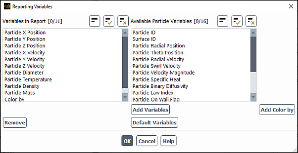
In the Reporting Variables dialog box (Figure 24.68: The Reporting Variables Dialog Box), you can change the variables in the report. The list under Variables in Report contains all variables currently reported. The list under Particle Variables contains the particle variables that are available for you to select. You can use the following buttons to modify the Variables in Report list:
: Removes selected variables from that list.
: Restores the default list.
: Adds selections to the report using.
: Adds the Color by variable to the list of Variables in Report, which is the only way to get cell values or customized field functions into the report.
Important: Note that it is possible to select one variable in the Reporting Variables dialog box and a variable from the Color by drop-down list in the Particle Tracks dialog box, however, each variable is reported only once.
Click the button and specify a file name for the step-by-step report file in The Select File Dialog Box.
A detailed report similar to the following example will be saved to the specified file before the trajectories are plotted. (You may also choose to print the report in the console by choosing Console as the Report to option and clicking or , but the report is very long that it is unlikely to be of use to you in that form.)
 FILE  TYPE: 1
 COLUMNS:  11
 TITLE: TRACK  HISTORY

 COLUMN  TYPE  VARIABLE                          (UNITS)
 ------  ----  --------                          -------
      1     2  ParticleResidenceTime             (s)
      2    10  ParticleXPosition                 (m)
      3    10  ParticleYPosition                 (m)
      4    10  ParticleZPosition                 (m)
      5    10  ParticleXVelocity                 (m/s)
      6    10  ParticleYVelocity                 (m/s)
      7    10  ParticleZVelocity                 (m/s)
      8    10  ParticleDiameter                  (m)
      9    10  ParticleTemperature               (K)
     10    10  ParticleDensity                   (kg/m3)
     11    10  ParticleMass                      (kg)
---------------------------------------------

  0.00000e+00   5.00000e-02   5.00000e-02   5.00000e-02   2.00000e+01   0.0000  .  .  .
  1.07087e-07   5.00000e-02   5.00000e-02   5.00000e-02   1.23339e+01   2.6696  .  .  .
  2.51617e-07   5.00000e-02   5.00000e-02   5.00000e-02   1.04417e+01   3.3286  .  .  .
 .              .             .             .             .            .
 .              .             .             .             .            .
 .              .             .             .             .            .
The default step-by-step report lists the position, velocity, diameter, temperature, density and mass of the particle at selected time steps along the trajectory. In addition, the variable you have selected in the Color by list is also included. If you choose Console as the Report to option, the variable names are written as the header of each column. (You may need to use the scroll bar to view all variables in this column.)
Time       X-Position   Y-Position   Z-Position    X-Velocity   Y-Velocity    Z-Veloc
0.000e+00  1.000e-03    3.120e-02    0.000e+00    1.000e+01     5.000e+00     0.000e
1.672e-05  1.168e-03    3.128e-02    0.000e+00    1.010e+01     4.988e+00     0.000e
3.342e-05  1.337e-03    3.137e-02    0.000e+00    1.019e+01     4.977e+00     0.000e
5.010e-05  1.508e-03    3.145e-02    0.000e+00    1.028e+01     4.965e+00     0.000e
6.675e-05  1.680e-03    3.153e-02    0.000e+00    1.038e+01     4.954e+00     0.000e
8.338e-05  1.854e-03    3.161e-02    0.000e+00    1.047e+01     4.942e+00     0.000e
.          .            .            .            .             .             .
.          .            .            .            .             .             .
.          .            .            .            .             .             .
If you change the reporting variables, only those selected will appear in the report. The particle time is always reported in the first column. Note that it is possible to select one variable in the Reporting Variables dialog box and a variable from the Color by drop-down list in the Particle Tracks dialog box, however, each variable is reported only once.
When the report is written to a file, a table at the beginning of the file lists all variables selected with the corresponding unit. Thus you can display or export any variable along a particle trajectory to the console or to a file.
Note that the Coarsen option affects the step-by-step report.
In transient cases, when using unsteady tracking, you may want to obtain a report of the current positions and states of the particles. Selecting Current Positions under Report Type in the Particle Tracks Dialog Box enables the export of the current positions of the particles.
The procedure for generating files containing current position reports is listed below:
Follow steps 1 and 2 in Displaying of Trajectories for displaying trajectories. You may want to track only one particle stream at a time, using the Track Single Particle Stream option.
Select Current Position as the Report Type (Reporting group box).
Select File as the Report to option. (The button will become the button.)
In the Significant Figures field, enter the number of significant figures to be used in the report.
To choose the variables to be included in the report, click the button.
This button is not available when Sample File Format is selected.
In the Reporting Variables dialog box (Figure 24.68: The Reporting Variables Dialog Box), you can change the variables in the report. The list under Variables in Report contains all variables currently reported. The list under Particle Variables contains the particle variables that are available for you to select. You can use the following buttons to modify the Variables in Report list:
: Removes selected variables from that list.
: Restores the default list.
: Adds selections to the report.
: Adds the Color by variable to the list of Variables in Report, which is the only way to get cell values or customized field functions into the report.
Important: Note that it is possible to select one variable in the Reporting Variables dialog box and a variable from the Color by drop-down list in the Particle Tracks dialog box, however, each variable is reported only once.
If you want to generate a file containing the particle current positions in the same file format that is used for particle sampling, select Sample File Format.
The generated file can be used as an injection file to transfer a population of particle parcels from one simulation into another (see below for details). It is also possible to use this file in a case with a different mesh.
Click the button and specify a file name for the current position report file in The Select File Dialog Box.
The default current position report lists the position, velocity, diameter, temperature, density, mass and number in parcel of the particle at selected time steps along the trajectory. In addition, the variable you have selected in the Color by list is also included. If you change the reporting variables, only those selected will appear in the report. The particle time is always reported in the first column. It is possible to select one variable in the Reporting Variables dialog box and a variable from the Color by drop-down list in the Particle Tracks dialog box, however, each variable is reported only once.
The output to a file or to the console has the same format as the step-by-step report for steady-state cases.
Time       X-Position  Y-Position  Z-Position   X-Velocity   Y-Velocity  Z-Velocity
0.000e+00  1.000e-03   3.120e-02   0.000e+00    1.000e+01    5.000e+00    0.000e+00
1.672e-05  1.168e-03   3.128e-02   0.000e+00    1.010e+01    4.988e+00    0.000e+00
3.342e-05  1.337e-03   3.137e-02   0.000e+00    1.019e+01    4.977e+00    0.000e+00
5.010e-05  1.508e-03   3.145e-02   0.000e+00    1.028e+01    4.965e+00    0.000e+00
6.675e-05  1.680e-03   3.153e-02   0.000e+00    1.038e+01    4.954e+00    0.000e+00
8.338e-05  1.854e-03   3.161e-02   0.000e+00    1.047e+01    4.942e+00    0.000e+00
.          .            .          .            .            .            .
.          .            .          .            .            .            .
.          .            .          .            .            .            .
Also listed are the diameter, temperature, density, mass of the particles, number in parcel and the variable selected from the Color by list. (You may need to use the scroll bar to view this information.)
Time       Diameter    Temperature   Density     Mass        Number      ColorBy
9.999e-04  9.352e-05   3.710e+02     6.840e+02   2.929e-10   2.792e+02   4.783e-02
1.999e-03  7.952e-05   3.710e+02     6.840e+02   1.801e-10   2.792e+02   3.834e-02
3.000e-03  6.660e-05   3.710e+02     6.840e+02   1.058e-10   2.792e+02   2.989e-02
4.001e-03  5.425e-05   3.710e+02     6.840e+02   5.719e-11   2.792e+02   3.719e-02
5.001e-03  4.184e-05   3.710e+02     6.840e+02   2.624e-11   2.792e+02   2.978e-02
.          .           .             .           .           .           .
.          .           .             .           .           .           .
.          .           .             .           .           .           .
If you selected Sample File Format, then the report file also includes
the flow-time column. This column contains the current simulated time
at which the report was written. When using the file to transfer a population of particle
parcels into another simulation, you can use the Start Time and
Start Flow-Time in File file injection point properties in the
Set Injection Properties dialog box to control the particle injection
time. For example, if you set Start Flow-Time in File to a value that is
only minimally lower than the flow-time, then the particle parcels will
be injected into the domain at the specified Start Time.
Ansys Fluent reports the magnitudes of the interphase exchange of momentum, heat, and mass in each control volume in your Ansys Fluent model. You can display these variables graphically, by drawing contours, profiles, and so on. They are all contained in the Discrete Phase Sources... category of the variable selection drop-down list that appears in postprocessing dialog boxes:
DPM Mass Source
DPM X,Y,Z Momentum Source
DPM Swirl Momentum Source
DPM Turbulent Kinetic Energy Source
DPM Turbulent Dissipation Source
DPM Sensible Enthalpy Source
DPM Enthalpy Source
DPM Burnout
DPM Evaporation/Devolatilization
DPM (species) Source
DPM Mixture Fraction Source
DPM Mixture Fraction Secondary Source
DPM Inert Source
See Field Function Definitions for definitions of these variables.
Note that these exchange terms are updated and displayed only when coupled calculations are performed. Displaying and reporting particle trajectories (as described in Displaying of Trajectories and Particle Tracking Statistics) will not affect the values of these exchange terms.
The exchange terms are reported as the rate occurring in each cell. A unit cell depth is used for 2D cases, and a reference cell depth of 1 radian is used for 2D axisymmetric cases.
In Ansys Fluent, the discrete phase variables listed in the tables below can be used for:
coloring the particle trajectories
step-by-step reporting (see Step-by-Step Reporting of Trajectories)
reporting of the current position and states of unsteady particles (see Reporting of Current Positions for Unsteady Tracking)
The following variables are available for all DPM simulations.
Table 24.7: General Particle Variables
| Name | Symbol Name in Journals | Units | Description |
|---|---|---|---|
| Particle Residence Time |
particle-resid-time
| time | Time since the moment of particle injection. |
| Particle ID |
particle-id
| - | Unique (global) particle ID. |
| Surface ID |
surface-id
| - | ID of the surface from which the particle was released; else -1. |
| Particle X Position |
particle-x-position
| length | Particle position in the global X-direction. |
| Particle Y Position |
particle-y-position
| length | Particle position in the global Y-direction. |
| Particle Z Position |
particle-z-position
| length | (3d only) Particle position in the global Z-direction. |
| Particle Radial Position |
particle-radial-position
| length | (3d only) Particle radial coordinate w.r.t. the cylindrical coordinate system defined for the reference thread. |
| Particle Theta Position |
particle-theta-position
| angle | (3d only) Particle theta coordinate w.r.t. the cylindrical coordinate system defined for the reference thread, angle counted starting from a plane containing the Y axis. |
| Particle X Velocity |
particle-x-velocity
| velocity | Particle velocity component in the global X-direction. |
| Particle Y Velocity |
particle-y-velocity
| velocity | Particle velocity component in the global Y-direction. |
| Particle Z Velocity |
particle-z-velocity
| velocity | (3d only) Particle velocity component in the global Z-direction. |
| Particle Radial Velocity |
particle-radial-velocity
| velocity | (3d only) Particle radial velocity component w.r.t. the cylindrical coordinate system defined for the reference thread. |
| Particle Swirl Velocity |
particle-swirl-velocity
| velocity | (3d only) Particle swirl velocity component w.r.t. the cylindrical coordinate system defined for the reference thread. |
| Particle Velocity Magnitude |
particle-velocity-mag
| velocity |

|
| Particle Diameter |
particle-diameter
| length | Particle diameter,  . . |
| Particle Density |
particle-density
| density | Particle mass density,  . The density may be defined as a function of temperature. For
multicomponent particles, it can be calculated as a volume-weighted value of the density of
the droplet components. . The density may be defined as a function of temperature. For
multicomponent particles, it can be calculated as a volume-weighted value of the density of
the droplet components. |
| Particle Specific Heat |
particle-Cp
| specific-heat | Particle-specific heat capacity defined in material settings for the current particle temperature (or at the reference temperature if physical property averaging is used). |
| Particle Binary Diffusivity |
particle-binary-diffusivity
| diffusivity |
|
| Particle Mass |
particle-mass
| mass |

|
| Particle Temperature |
particle-temperature
| temperature | Particle temperature,  (300 K if particle temperature is not solved). (300 K if particle temperature is not solved). |
| Particle Law Index |
particle-law-index
| - | Current law index number:
|
| Particle On Wall Flag |
particle-on-wall
| - | True (1) if the particle is a film particle. |
| Particle Reynolds Number |
particle-reynolds-number
| - |

|
| Particle Time Step |
particle-time-step
| time | Time step used by the numerical integration scheme. |
| Particle Number in Parcel |
particle-number-in-parcel
| mass per time / non-dimensional |
|
| Tracking Scheme |
tracking-scheme
| - |
|
| Number of Refinements |
number-of-refinements
| - | Number of times by which the integration time step size was reduced in the adaptive integration scheme. |
| Particle Penetration |
particle-penetration
| length | Distance traveled by the parcel from the injection reference position. |
| Parcel Mass |
parcel-mass
| mass | (Unsteady tracking only) Mass of Parcel = Mass of Particle x Number of Particles per Parcel. |
| Parcel Diameter |
parcel-diameter
| length | (Unsteady tracking only) Parcel diameter computed from parcel mass and parcel density. |
| Parcel Volume |
parcel-volume
| volume | (Unsteady tracking only) Volume of Parcel = Volume of Particle x Number of Particles per Parcel. |
| Particle Current Time |
particle-current-time
| time | (Unsteady tracking only) Particle time (identical to the current flow time). |
The following variables are available if particle heat/mass transfer is enabled.
Table 24.8: Particle Variables with Heat and Mass Transfer
| Name | Symbol Name in Journals | Units | Description |
|---|---|---|---|
| Latent Heat |
latent-heat
| specific-energy | Particle latent heat at the current particle temperature. |
| Vaporization Limiting Time |
vaporization-limiting-time
| time |
Time scale for achieving fractional changes in both particle mass and temperature according to the Vaporization Limiting Factors specified in the Discrete Phase Model dialog box. This is available when Droplet or Multicomponent particles are not enabled in the Coupled Heat-Mass Solution group box in the Discrete Phase Model dialog box (Numerics tab). |
| Particle Lewis Number |
particle-lewis-number
| - |
(Droplet particles only) 
|
| Particle Nusselt Number |
particle-nusselt-number
| - |
Nusselt Number: Ranz-Marshall 
|
| Bt Heat Transfer Number |
bt-heat-transfer-number
| - | (Droplet particles only) Spalding heat transfer number (Equation 12–96 in the Fluent Theory Guide). |
| Bm Mass Transfer Number |
bt-mass-transfer-number
| - | (Droplet particles only) Spalding mass transfer number (Equation 12–86 in the Fluent Theory Guide). |
Mass Fraction of species-n
| - | (Combusting particles with multiple surface reactions only) Mass fraction of the solid species as defined in the Selected Solid Species list in the Species dialog box. | |
Particle Mass Fraction of species-n
| - | (Multicomponent particles only) Mass fraction of the liquid component. | |
| Particle Enthalpy | specific-energy | Particle enthalpy at the current particle temperature. For multicomponent particles, it is calculated as a mass-weighted value of the enthalpies of the droplet components. | |
| Particle Liquid Mass Fraction |
particle-liquid-mass-fraction
| - |
|
| Particle Volatile Mass Fraction |
particle-volatile-fraction
| - |
|
| Particle Char Mass Fraction |
particle-char-fraction
| - | (Combusting particles only) Mass fraction of the char component of the particle. |
The following variables are available if the DEM model is enabled.
Table 24.9: Particle Variables with the DEM model
| Name | Symbol Name in Journals | Units | Description |
|---|---|---|---|
| Total X Force |
force-x-total
| force | X component of the total force (body force and volume force) acting on the DEM
particle during the DEM collision:
|
| Total Y Force |
force-y-total
| force | Y component of the total force (body force and volume force) acting on
the DEM particle during the DEM collision:
|
| Total Z Force |
force-z-total
| force | Z component of the total force (body force and volume force) acting on
the DEM particle during the DEM collision:
|
| Total Force Magnitude |
force-total-mag
| force |

|
| Collision X Force |
force-x-coll
| force | X component of the body force acting on the DEM particle during the DEM
collision:
|
| Collision Y Force |
force-y-coll
| force | Y component of the body force acting on the DEM particle during the DEM
collision:
|
| Collision Z Force |
force-z-coll
| force | Z component of the body force acting on the DEM particle during the DEM
collision:
|
| Collision Force Magnitude |
force-coll-mag
| force |

|
| Total X Acceleration |
acc-x-total
| acceleration | X component of total acceleration due to the total force during the DEM
collision:
|
| Total Y Acceleration |
acc-y-total
| acceleration | Y component of total acceleration due to total Force during DEM
collision:
|
| Total Z Acceleration |
acc-z-total
| acceleration | Z component of total acceleration due to the total force during the DEM
collision:
|
| Total Acceleration Magnitude |
acc-total-mag
| acceleration |

|


The following variables are available if particle rotation is enabled.
Table 24.10: Particle Variables with Particle Rotation
| Name | Symbol Name in Journals | Units | Description |
|---|---|---|---|
| Angular X Velocity |
x-angular-velocity
| angular velocity | Particle rotation rate about the X-axis. |
| Angular Y Velocity |
y-angular-velocity
| angular velocity | Particle rotation rate about the Y-axis. |
| Angular Z Velocity |
z-angular-velocity
| angular velocity | Particle rotation rate about the Z-axis. |
| Angular Velocity Magnitude |
angular-velocity-mag
| angular velocity |

|
The following variables are available if user define particles are enabled.
Table 24.11: Particle Variables with User-Defined Particles
| Name | Symbol Name in Journals | Units | Description |
|---|---|---|---|
User Value i
|
user-value-
| - | User data stored in TP_USER_REAL(tp,
. See
DEFINE_DPM_SCALAR_UPDATE
in the Fluent Customization Manual for an
example. |
The following variables are available if particle breakup is enabled.
Table 24.12: Particle Variables with Particle Breakup
| Name | Symbol Name in Journals | Units | Description |
|---|---|---|---|
| Particle Breakup Type |
particle-breakup-type
| - |
|
| Particle Weber Number Gas |
particle-weber-number-gas
| - | Liquid Weber number based on gas density 
|
| Particle Weber Number Liquid |
particle-weber-number-liquid
| - | Liquid Weber number based on particle density 
|
| SSD break up time |
ssd-break-up-time
| time | Equation 12–445 in the Fluent Theory Guide |
| Normalized TAB displacement |
normalized-TAB-displacement
| - | Equation 12–405 in the Fluent Theory Guide |
| Normalized TAB velocity |
normalized-TAB-velocity
| 1/time | Equation 12–409 in the Fluent Theory Guide |
| WAVE break up time |
WAVE-break-up-time
| time | Equation 12–437 in the Fluent Theory Guide |
| WAVE mass in shed drops |
WAVE-mass-in-shed-drops
| mass | Mass of the shed-off droplet during the WAVE breakup process. |
| WAVE shed drops cutoff mass |
WAVE-shed-drops-cutoff-mass
| mass |
Cut-off mass for the shed particles. During WAVE breakup, a new parcel will be created if the particle shed mass becomes larger than the cutoff mass. |
| Accumulated break up time |
accumulated-break-up-time
| time | |
| PILCH_ERDMAN deformation time |
PILCH_ERDMAN-deformation-time
| time | Equation 12–448 in the Fluent Theory Guide |
| PILCH_ERDMAN break up time |
PILCH_ERDMAN-break-up-time
| time | Equation 12–449 in the Fluent Theory Guide |
| PILCH_ERDMAN total break up time |
PILCH_ERDMAN-total-break-up-time
| time | Equation 12–455 in the Fluent Theory Guide |
| PILCH_ERDMAN initial weber number |
PILCH_ERDMAN-initial-weber-number
| - | Particle Weber number at the beginning of the Pilch-Erdman breakup process. It is used to compute the deformation and breakup time of the droplets. |
| PILCH_ERDMAN initial diameter |
PILCH_ERDMAN-initial-diameter
| length | Particle diameter at the beginning of the Pilch-Erdman breakup process. |
| MADABHUSHI column break up time |
MADABHUSHI-column-break-up-time
| time | Equation 12–447 in the Fluent Theory Guide |
Ansys Fluent reports various discrete phase particle/parcel quantities including erosion/accretion rates, radiation quantities, and (optionally) cell-averaged particle size, velocity, temperature, and so on. You can display these variables graphically, by drawing contours, profiles, and so on. They are accessed in the Discrete Phase Variables... category of the variable selection drop-down list that appears in postprocessing dialog boxes.
Several quantities are automatically available depending on the models being used in the simulation. For the cell-averaged quantities to be available, you must first enable Mean Values under Contour Plots for DPM Variables in the Discrete Phase Model dialog box, Discrete Phase Model Dialog Box. RMS quantities are also available for particle velocity and temperature by enabling RMS Values.
Note: Enabling Mean Values to track the cell-averaged variables will increase the memory requirements of your simulation.
The following lists specify those variables that are available automatically and those that require you to enable them
Variables available automatically
DPM Erosion Rate (Generic)
DPM Erosion Rate (Finnie)
DPM Erosion Rate (McLaury)
DPM Erosion Rate (Oka)
DPM Erosion Rate (DNV)
DPM Erosion Rate (Wall Shear)
DPM Accretion Rate
DPM Absorption Coefficient
DPM Emission
DPM Scattering
DPM Concentration
DPM Wall X Force
DPM Wall Y Force
DPM Wall Z Force
DPM Wall Normal Pressure
DPM (species) Concentration
DPM Collision Rate
Particle rotation variables (Particle rotation simulations only)
Angular X Velocity
Angular Y Velocity
Angular Z Velocity
Angular Velocity Magnitude
Angular Velocity (in the Particle Vector Style dialog box)
Cell-averaged variables available when Mean Values are enabled
DPM Volume Fraction
DPM Particles in Cell
DPM Parcels in Cell
DPM Number Density
DPM X, Y, Z Velocity
DPM Diameter
DPM Density
DPM Temperature
DPM Enthalpy
DPM Specific Heat
DPM D20
DPM D30
DPM D32
DPM D43
DPM Granular Temperature
DPM Conc. of (component)
For the discrete phase variable  , the event-based time average (mean) in a cell is calculated as:
 | (24–23) |
where
 = number of parcels in the cell = number of parcels in the cell |
 = number of particles in the = number of particles in the  th parcel
 |
 = residence time of the parcel = residence time of the parcel |
RMS variables available when Mean Values and RMS Values are enabled
DPM RMS X, Y, Z Velocity
DPM RMS Temperature
DPM RMS Diameter
The RMS value of the discrete phase variable  is calculated as:
 | (24–24) |
See Field Function Definitions for definitions of these variables.
Note that these variables are updated and displayed only when coupled calculations are performed. Displaying and reporting particle trajectories (as described in Displaying of Trajectories and Particle Tracking Statistics) will not affect the values of these variables.
Note: If you select Enable Node Based Averaging in the Numerics tab of the Discrete Phase Model dialog box, any previously calculated DPM variables will be rendered useless and need to be recomputed.
If you are performing a transient simulation, you can include the computation of unsteady time statistics (mean and RMS) for the discrete phase(s) of the transient flow. These are computed on a per-phase basis by event-based time averaging over the discrete phase parcels in the domain. This means that the sampling of the discrete phase particle quantity in a given cell occurs when (and only when) a parcel passes through the cell.
To calculate the unsteady DPM time statistics, enable Data Sampling for Time Statistics in the Run Calculation task page and enable DPM Variables in the Sampling Options dialog box when preparing to run your simulation (see Inputs for Time-Dependent Problems).
For a discrete phase variable,  , the event-based time average (mean) in a cell is calculated from Equation 24–25.
 | (24–25) |
where  is the number of parcels in the cell, and
 | (24–26) |
Here  is the number of particles in the
  th parcel and
  is the residence time of the
  th parcel in the cell. The weighting by residence time is necessary
because a parcel may pass through more than one cell within a computational time step and
therefore its contribution to the averaged cell quantities depends on the fraction of the time
step spent in each cell.
th parcel in the cell. The weighting by residence time is necessary
because a parcel may pass through more than one cell within a computational time step and
therefore its contribution to the averaged cell quantities depends on the fraction of the time
step spent in each cell.
The time-averaged DPM volume fraction is calculated from the individual number of particles in the parcel, the particle volume, and its residence time in the cell in relation to the individual time step.
The RMS value is also available and is computed from Equation 24–27.
 | (24–27) |
Note that these quantities are averaged over all parcels that have passed through the cell and are therefore different from the instantaneous cell-averaged values described in Reporting of Discrete Phase Variables.
Below is a list of the available unsteady statistics when DPM Variables is enabled in the Sampling Options dialog box. These are accessible by selecting the Unsteady DPM Statistics... category in postprocessing or reporting dialog boxes. Note that the availability of some quantities depends on the physics models being used. For definitions of these quantities, refer to the definitions of the instantaneous quantities from which they are derived (see Alphabetical Listing of Field Variables and Their Definitions).
Unsteady DPM Statistics
Mean DPM Volume Fraction
Accum DPM Particles in Cell
Mean DPM X, Y, Z Velocity
Mean DPM Diameter
Mean DPM Density
Mean DPM Temperature
Mean DPM Granular Temperature
Mean DPM Number Density
Accum DPM Parcels in Cell
Mean DPM D20
Mean DPM D30
Mean DPM D32
Mean DPM D43
RMS DPM Volume Fraction
RMS DPM X, Y, Z Velocity
RMS DPM Diameter
RMS DPM Density
RMS DPM Temperature
RMS DPM Granular Temperature
RMS DPM Number Density
Explanations for the Accum... variables are provided in Alphabetical Listing of Field Variables and Their Definitions.
Particle states (position, velocity, diameter, temperature, and mass flow rate) can be written to files at various boundaries and planes (lines in 2D) using the Sample Trajectories Dialog Box (Figure 24.69: The Sample Trajectories Dialog Box).
![]() Results → Reports → Discrete Phase → Sample
Results → Reports → Discrete Phase → Sample![]() Edit...
Edit...
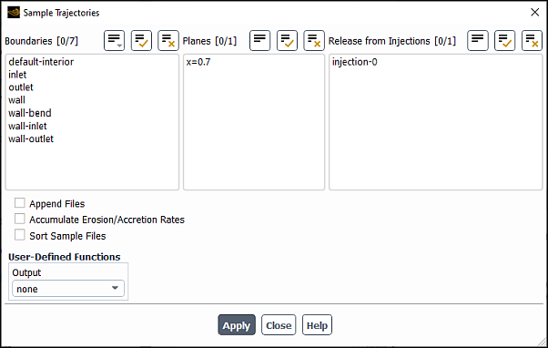
The procedure for generating files containing the particle samples is listed below:
Select the injections to be tracked in the Release From Injections list.
Select the surfaces at which samples will be written. These can be boundaries from the Boundaries list or planes from the Planes list (in 3D) or lines from the Lines list (in 2D).
If you want to use the particle sampling file as an unsteady injection file, select Sort Sample Files.
The Sort Sample Files option causes the sample files to be sorted in a reproducible manner. For steady particle tracking, files will be sorted first by injection and then by particle ID. For unsteady particle tracking, the files will be sorted strictly by the simulated time (
flow-timein the 13th column in the sample file) at which the particle passes the sampling plane surface or mesh zone.Click the button. Note that for unsteady particle tracking, the button will become the button (to initiate sampling) or a button (to stop sampling).
Clicking the button will cause the particles to be tracked and their status to be written to files when they encounter selected surfaces. The file names will be formed by appending
.dpmto the surface name. The files can be used for:Postprocessing probability distributions of particle properties (see Histogram Reporting of Samples)
Injecting particles using the file injection type
Note: If you select a face zone in a mesh interface for sampling, Fluent will sample the particles on both of the interface zones and will write out a total of three files. Two of these files correspond to the particles that encounter each respective interface zone from upstream. The third file contains the complete set of particles that have crossed the mesh interface pair (via either interface zone).
For unsteady particle tracking, clicking the button will open the files and write the file header sections. If the solution is advanced in time by computing some time steps, the particle trajectories will be updated and the particle states will be written to the files as they cross the selected planes or boundaries. Clicking the button will close the files and end the sampling.
For stochastic tracking, it may be useful to repeat this process multiple times and append the results to the same file, while monitoring the sample statistics at each update. To do this, enable the Append Files option before repeating the calculation (clicking ). Similarly, you can cause erosion and accretion rates to be accumulated for repeated trajectory calculations by turning on the Accumulate Erosion/Accretion Rates option. (See also Postprocessing of Erosion/Accretion Rates.)
The format and the information written for the sample output can also be controlled through
a user-defined function, which can be selected in the Output drop-down
list. See
DEFINE_DPM_OUTPUT
in the Fluent Customization Manual for more
information.
The generated sample files can be used as injection file in a file injection. Both files use the same file formats which differ between steady and unsteady particle tracking. For details, see Point Properties for File Injections.
If the number of lines in the sampling file is large, you can reduce it by combining sets of similar line entries into one single entry per such set. The mass represented by that entry will be increased accordingly to ensure mass conservation. For details, see Data Reduction of Samples.
DPM sample files can be created using the Sample Trajectories Dialog Box (as described in Sampling of Trajectories) or by the VOF-to-DPM model transition mechanism. Such a file contains multiple records, each consisting of values for the same set of variables. You can postprocess probability distributions and simple correlation analyses of these variables using the Trajectory Sample Histograms Dialog Box (Figure 24.70: The Trajectory Sample Histograms Dialog Box).
![]() Results → Reports
→ Discrete Phase
→ Histogram
Results → Reports
→ Discrete Phase
→ Histogram![]() Edit...
Edit...
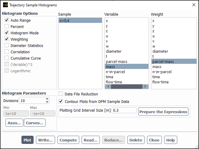
The basic procedure for plotting a histogram of the probability distribution of a variable read from data in a sample file is listed below:
Select a sample file to be read by clicking the button. After you read in the sample file, the sample name will appear in the Sample list.
Select the data sample in the Sample list, and then select the variable for which to plot the probability distribution histogram from the Variable list.
Select the variable by which to weight the file individual line entries from the Weight list. To obtain representative information for most intensive variables, such as temperature, velocity, or position, you should select:
mass-flow for a sample file from steady-state particle tracking
parcel-mass for a sample file from unsteady particle-tracking.
If the sampled particle streams / parcels all have the same flow rate / parcel mass, you can clear Weighting.
You can specify the number of bins, or intervals, in the plot in the Divisions field under Histogram Parameters.
If you want to plot just some part of the probability distribution, clear Auto Range and specify the range of values in the Min and Max fields under Histogram Parameters. You can reset Min and Max to the complete range by clicking .
If variable values you are investigating span several orders of magnitude, you can use logarithmic scaling of the bins by selecting Logarithmic under Histogram Options. Note that this option is available only for the variables that take only positive values. With this option, you should select the logarithmic scaling format for the abscissa and, if necessary, for the ordinate in the Axes dialog box that opens by clicking Axes… (Histogram Parameters group box).
Click the button at the bottom of the dialog box to display the histogram in the graphics window.
In addition, the following controls are available:
Percent
By default, the percentages of the total amount measured by the weighting variable will be plotted on the
 axis. You can plot the actual number of sampled particle streams / parcels
(that is, line entries from the file that fall into each interval on the
axis. You can plot the actual number of sampled particle streams / parcels
(that is, line entries from the file that fall into each interval on the  axis) by clearing Percent under Histogram
Options. If Weighting is selected, the sum of the weights of
all entries in each bin will be plotted instead of the number.
axis) by clearing Percent under Histogram
Options. If Weighting is selected, the sum of the weights of
all entries in each bin will be plotted instead of the number.Histogram Mode
To display a probability density function curve instead of the histogram, clear Histogram Mode under Histogram Options. You can enable the display of data point markers in the plot using the Curves dialog box that opens by clicking Curve....
Diameter Statistics
If you want to display in the console a summary for the selected variables similar to that in Summary Reporting of Current Particles, select Diameter Statistics and click . Although these statistics are computed for any selected variable in the Variable list, it is applicable only to the diameter information.
If you want to further postprocess the plot data with other software tools, you can store them in an XY-plot file format using the button. If you use the default filename extension .his, the file be written with a header. The header lines begin with the comment character
;and contain the same statistical information that is printed to the Fluent console when you click Plot.Delete
If you want to remove the currently highlighted sample from the Sample list and delete it from the Ansys Fluent session memory, but not the corresponding file, click Delete.
Correlation
When investigating the behavior of particles, it is sometimes desirable to know how one particle variable correlates with another particle variable. To facilitate this, the Correlation option exists. When you enable this option, an additional column of sampled variables appears, allowing you to choose the correlation variable (see Figure 24.71: The Trajectory Sample Histograms Dialog Box: Correlation). In this mode, every ordinate value will be a weighted average of the values of the correlation variable in all entries that fall into the respective bin.
Cumulative Curve
If you want to plot the continuous cumulative distribution function, enable the Cumulative Curve option. A cumulative distribution curve is computed of the variable that is selected in the Variable list using the weighting options. However, if the Correlation option is enabled along with the Cumulative Curve, then the cumulative curve of the variable selected in the Correlation list is plotted. For a constant particle density, you can plot a correlation curve for the particle mass by selecting the diameter as a Correlation variable and enabling (Variable)ˆ3. This calculates cubes of the variable chosen under Correlation and for which an average is calculated within each bin and used for the ordinate value in the plot as explained above.
Contour Plots from DPM Sample Data
If you want to use data from a sample file for graphical postprocessing (contour plotting) on the planar surface where the DPM particles were sampled, enable Contour Plots from DPM Sample Data and follow steps outlined in Contour Plots of DPM Particle Sampling Results on a Planar Surface.
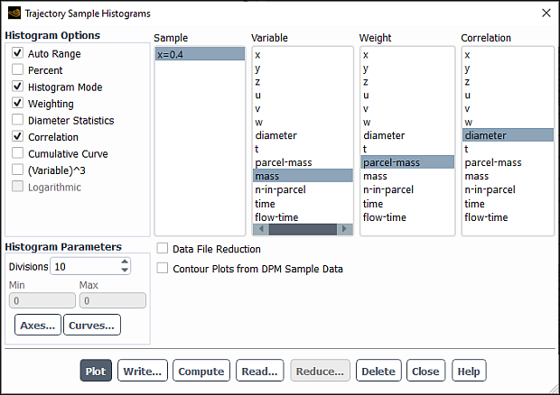
When you use a sample file as an injection file in a subsequent simulation, it may be desirable to reduce the number of particles injected by the file in order to lower the computational cost. In Ansys Fluent this can be done by reducing the number of lines the sample file contains using a method that is similar to that used to create a histogram. However, unlike a histogram, the weighted entries from the sample file are sorted into intervals for all variables simultaneously, not one variable at a time.
The method first sorts all file entries into groups, or bins, of entries that are sufficiently similar in all properties. The entries that have fallen into the same bin are then averaged to create a single entry. Conservation of mass and volume as well as the number of particles is achieved by appropriate weighting in the averaging process.
To reduce a sample file size:
Read a sample file as described in Analysis, Investigation, and Reporting of Samples.
Select the data sample in the Sample list.
Select Data File Reduction.
The Trajectory Sample Histograms dialog box will expand to show the Scale, No. of Bins list (between the Variable and Weight lists) and data file reduction inputs.
For each variable in the Variable list, specify the following parameters in the Data Reduction in the Selected Variable group box:
- 1st Bin Min , Last Bin Max
limit the range of values to consider. Note that the complete range for the selected variable is displayed in the Min and Max fields in the Histogram Parameters group box. You can use the Reset button to reset 1st Bin Min and Last Bin Max to their original values.
- LOG Scale
enables the use of a logarithmic scale. The behavior of this option is analogous to the Logarithmic option in Histogram Options (see Analysis, Investigation, and Reporting of Samples). By default, the linear scaling is used. This option is available only if all values for the variable in the sample file are positive.
- No. of Bins
the number of groups into which the specified range for this variable is to be divided. If you want to neglect any variable, set No. of Bins to 1. If you want to set the value you specified for all variables, click Set No. of Bins for All Variable.
Once you have specified 1st Bin Min, Last Bin Max, and No. of Bins, you can click Update to see the Resulting Bin Size. If the LOG Scale is selected, the value shown in the Resulting Bin Size is the ratio for LOG Scale.
You can quickly review the inputs for the scaling and number of bins for each variable in the Scale, No. of Bins information list.
For a standard DPM sample file generated by Ansys Fluent, you should use the default weighting. However, if you want to reduce data in a file that does not contain the default header and variable columns that are present in a standard DPM sample file, you can select a weighting variable manually from the Weight list. If you do not want to use the weight, clear the Weighting option in the Data Reduction Options group box. Note that in both scenarios, the reduced sample file may not represent the same mass, volume, and flow rates of discrete phase.
If the original sample file was generated from unsteady particle tracking, you can reduce the unsteady sample file to a regular steady-state injection file by selecting the Create Steady from Unsteady check box in the Data Reduction Options group box. This option is available only for sample files from unsteady particle tracking.
Once you have configured the data reduction settings for all variables and selected the data reduction options, click .
In The Select File Dialog Box that opens automatically, enter the name of your reduced injection sample file.
The number of aggregated records will be reported in the Ansys Fluent console.
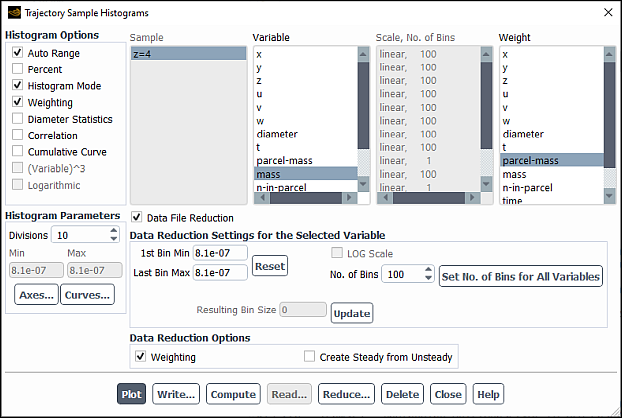
You can create contour plots of the spatial distribution of certain particle phase properties from DPM particle sampling on a specific planar surface (cut plane or planar domain boundary face zone). For example, you can create a contour plot of the droplet Sauter mean diameter on a plane orthogonal to the liquid spray direction. In this feature, the planar surface at which the DPM parcel samples are written to a file is divided into squares of a user-specified edge length. The DPM sampling events, which occur when particles cross the plane, are counted in each square. The weighted averages of different quantities are calculated based on the DPM particles sampled in that square. The results are then automatically interpolated into the CFD mesh and made available for graphical postprocessing as named expressions.
The procedural steps for using this feature are shown below.
Create a plane cutting through the geometry, or identify a planar domain boundary to be used. (See Plane Surfaces for details.)
Sample particle trajectories on the surface as described in Sampling of Trajectories.
A DPM sample file with the same name as the surface and a .dpm extension will be automatically saved in your working directory.
Results → Reports
→ Discrete Phase
→ Sample Edit...
In the Trajectory Sample Histograms dialog box, read the DPM sample file by using the Read... button. (See Figure 24.70: The Trajectory Sample Histograms Dialog Box.)
Results → Reports
→ Discrete Phase
→ Histogram Edit...
For more information about using the Trajectory Sample Histograms dialog box, see Histogram Reporting of Samples.
Enable Contour Plots from DPM Sample Data.
The Ansys Fluent solver automatically calculates a default value for Plotting Grid Interval Size, which determines the size of the squares into which the sampling plane is divided.
If necessary, adjust the Plotting Grid Interval Size.
When specifying the interval size, you should only use values that are larger than the local size of the mesh elements; otherwise, the calculation and interpolation may neglect data points and thus lose fidelity and accuracy. In addition, larger discretisation intervals reduce the risk that too few DPM sampling events fall within any given discretisation square of the plane, and, therefore, the local values for the quantities of interest will be shown as 0.
Conversely, a very large interval size can affect the accuracy of the calculation of mass flux (steady particle tracking) or mass per unit area (unsteady particle tracking) in regions where the surface either has a boundary or touches the domain boundary. This is because the calculation uses the size of the entire square, although there can be no sampling events outside the plane or domain boundaries.
Click .
The Ansys Fluent solver generates named expressions with names that contain the name of the particle sampling surface (represented by
<surfname>in the named expressions below).patt_significance_threshold: Is the minimum number of DPM sampling events required for statistical evaluation of the local values of quantities defined by the named expressions whose name contain _signif_ (see below). Each local value will be suppressed if this number is below the specified significance threshold. In this way, values that are based on insufficient statistical data (for example, at the periphery of a spray) are removed from plots.
The significance threshold is a constant single-valued expression that can be adjusted as desired.
<surfname>_number_of_events: Is the number of DPM sampling events (that is, entries in the *.dpm file) that have been combined into a single value for every quantity in the local square element of the discretized plane. This number is affected by the value you have entered for Plotting Grid Interval Size in the Trajectory Sample Histograms dialog box.Note that if this number is small, all other values in this location will have uncertainty and should not be used for comparison with experimental results nor for any evaluation of the simulation prediction.
<surfname>_sufficient_data_flag: Is a local indicator flag. A value of 1 is shown where the number of DPM sampling events combined into a single local data point exceeds the significance threshold, and a value of 0 is shown elsewhere. You can use this named expression to check if there were enough events in the sampling, and if the Plotting Grid Interval Size was sufficiently large.<surfname>_signif_sauter_mean_diameter: Is the local Sauter Mean Diameter [m].<surfname>_signif_mass_weighted_mean_temp.: Is the mass-weighted mean temperature [K].<surfname>_signif_mass_weighted_mean_vel._m: Is the mass-weighted mean velocity magnitude [m/s].<surfname>_signif_mass_per_unit_area: (unsteady particle tracking) Is the amount of DPM mass per unit area that has been calculated in the local square of the discretization plane [kg/m2].<surfname>_signif_mass_flux: (steady particle tracking) Is the mass flux that has been calculated in the local square of the discretization plane [kg/m2s].
Use the generated named expressions for graphical postprocessing (contour plotting). See Postprocessing Expressions for more information.
Important: You must make sure that the named expressions are postprocessed only on the planar surface for which they have been prepared, and whose name they bear. Otherwise, the visualisation will display incorrect data.
For many mass-transfer and flow processes, it is desirable to
know the mean diameter of the particles. A mean diameter,  , is calculated from the particle size distribution
using the following general expression [83]:
, is calculated from the particle size distribution
using the following general expression [83]:
 | (24–28) |
where  and
and  are integers and
  is the
distribution function (for example, Rosin-Rammler).
is the
distribution function (for example, Rosin-Rammler).  , for example, is the average (arithmetic) particle
diameter. The Sauter mean diameter (SMD),
, for example, is the average (arithmetic) particle
diameter. The Sauter mean diameter (SMD),  ,
is the diameter of a particle whose ratio of volume to surface area
is equal to that of all particles in the computation. A summary of
common mean diameters is given in Table 24.13: Common Mean Diameters and Their Fields of Application.
,
is the diameter of a particle whose ratio of volume to surface area
is equal to that of all particles in the computation. A summary of
common mean diameters is given in Table 24.13: Common Mean Diameters and Their Fields of Application.
Table 24.13: Common Mean Diameters and Their Fields of Application

|

| Order 
| Name | Field of Application |
|---|---|---|---|---|
| 1 | 0 | 1 | Mean diameter, 
| Comparisons, evaporation |
| 2 | 0 | 2 | Mean surface diameter, 
| Absorption |
| 3 | 0 | 3 | Mean volume diameter, 
| Hydrology |
| 2 | 1 | 3 | Overall surface diameter, 
| Adsorption |
| 3 | 1 | 4 | Overall volume diameter, 
| Evaporation, molecular diffusion |
| 3 | 2 | 5 | Sauter mean diameter, 
| Combustion, mass transfer, and efficiency studies |
| 4 | 3 | 7 | De Brouckere diameter, 
| Combustion equilibrium |
Summary information (number, mass, average diameter) for particles currently in the computational domain can be reported using the Particle Summary Dialog Box (Figure 24.73: The Particle Summary Dialog Box)
![]() Results → Reports → Discrete Phase → Summary
Results → Reports → Discrete Phase → Summary![]() Edit...
Edit...
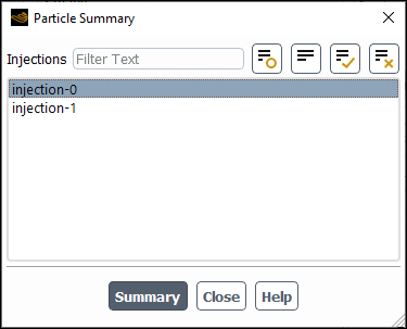
The procedure for reporting a summary for particle injections is as follows:
Select the particle injection(s) you want summarized in the Injections list.
Fluent provides a shortcut for selecting injections with names that match a specified pattern. To use this shortcut, enter the pattern in the Filter Text box. For example, if you specify
drop*, all injections that have names beginning with drop (for example, drop-1, droplet) will be listed.Click to display the injection summary in the console window.
   (*)-  Summary  for  Injection:  injection-0  -(*)

  Total  number  of  parcels              :  1862
  Total  number  of  particles            :  1.196710e+05
  Total  mass                             :  1.128303e-05 (kg)
  Maximum  RMS  distance  from  injector  :  7.372527e-01 (m)
  Maximum  particle  diameter             :  3.072739e-04 (m)
  Minimum  particle  diameter             :  1.756993e-06 (m)
  Overall  RR  Spread  Parameter          :  1.446806e+00
  Maximum  Error  in  RR  fit             :  1.071220e-01
  Overall  RR  diameter             (D_RR):  9.051303e-05 (m)
  Overall  mean  diameter           (D_10):  4.663269e-05 (m)
  Overall  mean  surface  area      (D_20):  5.344694e-05 (m)
  Overall  mean  volume             (D_30):  6.121478e-05 (m)
  Overall  surface  diameter        (D_21):  6.125692e-05 (m)
  Overall  volume  diameter         (D_31):  7.013570e-05 (m)
  Overall  Sauter  diameter         (D_32):  8.030141e-05 (m)
  Overall  De  Brouckere  diameter  (D_43):  1.082971e-04 (m)
You can calculate the erosion and accretion rates in a cumulative manner (over a series of injections) by using the Sample Trajectories dialog box. First select an injection in the Release From Injections list and compute its trajectory. Then enable the Accumulate Erosion/Accretion Rates option, select the next injection (after deselecting the first one), and click again. The rates will accumulate at the surfaces each time you click .
Important: Both the erosion rate and the accretion rate are defined at wall face surfaces only, so they cannot be displayed at node values.
Ansys Fluent provides functionality for assessing the solids deposition risk in the Selective Catalytic Reduction (SCR) process. The computation involves several chemical and hydrodynamic risk factors that are based on thermodynamic data and known chemical pathways, as well as on experimental evidence reported in the literature ([149], [156], [22], [133], and [176]). The risk assessment calculation should be invoked after the initial liquid film formation on the surfaces of the SCR device, and should cover a time period over one or more urea injection cycles. The risk variables are defined as dimensionless quantities that vary from 0 to 1, where 0 corresponds to no risk and 1 corresponds to maximum risk. Note that the risk assessment calculation is not a predictive model for urea deposit formation, and the obtained results should be considered only as rough guidance in exploring urea deposit formation trends.
The implementation takes into account the following chemistry risk factors:
Crystallization risk

The limiting urea mass fraction
 for the onset of crystallization is a function of film temperature
 ([149] and [133]). Therefore,
the crystallization risk over the time period
([149] and [133]). Therefore,
the crystallization risk over the time period  –
– can be calculated as the fraction of time when the urea mass fraction in
the liquid film
can be calculated as the fraction of time when the urea mass fraction in
the liquid film  exceeds
  :
:
(24–29)
Secondary reactions risk

According to [149], [156], and [22], the formation of biuret and/or cyanuric acid solids deposits starts at
 = 423-433 K and diminishes at
  = 523 K. In addition, the presence of HNCO in the gas phase above the film
is required. It follows that the secondary reactions risk over the time period
= 523 K. In addition, the presence of HNCO in the gas phase above the film
is required. It follows that the secondary reactions risk over the time period
 –
– can be calculated as the fraction of time when the liquid film is exposed
to a non-zero HNCO concentration and the film temperature is between
can be calculated as the fraction of time when the liquid film is exposed
to a non-zero HNCO concentration and the film temperature is between  and
and  as specified above.
(24–30)
In addition, the following hydrodynamic factors have been shown to affect solids deposit formation trends:
Intense dynamics can be quantified as fluctuations of film height [149]. When the fluctuations are high, the risk of deposit formation is impeded.
As reported by Smith et al. [149], thick film and high film velocity indicates low deposit formation risk, while Brack et al. [176] report that thick film and low heat flux indicate high deposit formation risk.
Accordingly, Ansys Fluent uses the following definitions to quantify the hydrodynamic risk factors:


Equation 24–31 and Equation 24–32 use the following nomenclature:
 = (Wall Film Height) / (Maximum Film Height) = (Wall Film Height) / (Maximum Film Height) |
 =(Wall Film Velocity) / (Maximum Wall Film Velocity) =(Wall Film Velocity) / (Maximum Wall Film Velocity) |
 = (Wall Film Heat Flux) / (Maximum Wall Film Heat Flux) = (Wall Film Heat Flux) / (Maximum Wall Film Heat Flux) |
Finally, averaging over the period from  to
to  and applying appropriate weighting factors, the total risk
  is calculated as:
 | (24–33) |
where:
 | (24–34) |
 | (24–35) |
The weighting factors  .
.  ,
,  , and
, and  are user-specified values.
You can access the functionality for assessing the risk of solids deposit formation via the following text commands:
define/models/dpm/options/scr-urea-deposition/enable-risk-analysis?
yes
You will be asked to define the wall zones where the risk assessment should be performed, for example:
Wall face zones(1) [()]
8
The implementation uses the data sampling and custom field functions in Ansys Fluent, and after enabling the risk assessment capability, the following steps are automatically performed:
Defining appropriate solution report definitions for calculating the maximum film height, velocity, and heat-flux.
Defining the required custom field functions for calculating the risk factors.
Enabling data sampling on the custom field functions.
Once the SCR urea deposition risk analysis is enabled, you can set the following parameters
and weighting factors (available under
define/models/dpm/options/scr-urea-deposition):
cryst-min-tempandcryst-max-temp: the minimum and maximum film temperatures for the onset of urea crystallization (K), respectivelycryst-min-mass-fract: the minimum urea mass fraction for the onset of urea crystallization as defined in [149] and [133]seco-rx-min-hnco: the minimum HNCO mass fraction in the gas phase above the liquid film for secondary reactions ( in Equation 24–30)
seco-rx-min-tempandseco-rx-max-temp: the minimum and maximum film temperatures for secondary reactions (K), respectively ( and
and  in Equation 24–30)
hydrodynamic-risk-weight: weighting factor for hydrodynamic risk ( in Equation 24–33)cryst-depo-weight: weighting factor for crystallization risk ( in Equation 24–34)velocity-based-risk-weight: weighting factor for velocity based risk ( in Equation 24–35)heat-flux-based-risk-weight: weighting factor for heat-flux based risk ( in Equation 24–35)wall-face-zones: wall zone list for solids deposit risk prediction
After the time-dependent calculation is completed, the following variables will be available under Custom Field Functions... category for post-processing:
scr-urea-overall-hydrodynamic-deposition-risk: is
 in Equation 24–35
scr-urea-overall-chemistry-deposition-risk: is
 in Equation 24–34
scr-urea-total-deposition-risk:
in Equation 24–33
Additional field variables reported under the Custom Field Functions... and SCR Urea Deposition Risk Analysis... categories are the following:
scr-urea-depo-risk-velocity-based (in the Custom Field Functions... category):
 in Equation 24–31
scr-urea-depo-risk-heat-flux-based (in the Custom Field Functions... category):
 in Equation 24–32
SCR Urea Crystallization Risk (in the SCR Urea Deposition Risk Analysis... category): is the chemistry based risk representation
in Equation 24–29
SCR Urea Secondary Reactions Risk (in the SCR Urea Deposition Risk Analysis... category): is the chemistry based risk representation
in Equation 24–30
SCR Overall Urea Chemical Deposition Risk (in the SCR Urea Deposition Risk Analysis... category): is the chemistry based risk representation
 in Equation 24–34
You may ignore the additional variables with the scr-urea-depo- prefix in the Custom Field Functions... category as they are intermediate quantities with no meaningful values.