The procedure for setting up and using the mesh morpher/optimizer for shape optimization is as follows:
Read the case into Ansys Fluent.
 File → Read
→ Case...
File → Read
→ Case...
If you want to use one of the built-in optimizers rather than specifying the deformation manually or using Design Exploration in Ansys Workbench to explore multiple deformation scenarios, you will need to provide an objective function in one of three ways: either as a user-defined function (UDF), a Scheme source file, or a customized function that is based on output parameters (that is, values from flux, force, surface integral, or volume integral reports). The goal of the optimizer is to deform the mesh in such a way that this objective function is minimized. Ansys Fluent will run the solution for a given design stage until convergence is reached, and then check to see if the objective function is satisfied. If the objective function is not satisfied, Ansys Fluent will proceed to the next design, and so on, until convergence is achieved from the point of view of the optimizer. You can specify the optimizer convergence criteria in step 12.d.iii.
Note that if you plan to use the newuoa optimizer, you must define the objective function as a UDF.
If you want to provide the objective function as a user-defined function (UDF), perform the steps that follow. For more information about UDFs, see the separate Fluent Customization Manual.
Write a UDF using the
DEFINE_ON_DEMANDmacro to define the objective function. The function name must beobjective_function. At the end of the objective function, the rpvarmorpher/objective_functionmust be set to the(current - target)value. It is this value that the optimizer will attempt to minimize.Compile the UDF using the Compiled UDFs dialog box. Make sure
libudfappears as the Library Name. User Defined →
User Defined →
Functions →
Compiled...
If you want to provide the objective function as a Scheme source file, perform the following steps:
Write a Scheme source file to define the objective function. The procedure name must be
objective-function. At the end of the objective function, the rpvarmorpher/objective-functionmust be set to the(current - target)value. It is this value that the optimizer will attempt to minimize.Load the Scheme source file (see Reading Scheme Source Files for details).
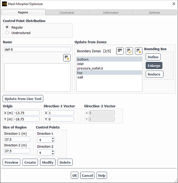
Open the Mesh Morpher/Optimizer dialog box by clicking in the Design ribbon tab (Parameter-Based group box).
The first time you click in a session, a question dialog box will ask you whether you want to enable the mesh morpher/optimizer. Click to load the libraries and open the Mesh Morpher/Optimizer dialog box (Figure 48.37: The Regions Tab of the Mesh Morpher/Optimizer Dialog Box).
Specify the manner in which you would like to define the locations of the control points, by making a selection from the Control Point Distribution list in the Regions tab of the Mesh Morpher/Optimizer dialog box (Figure 48.37: The Regions Tab of the Mesh Morpher/Optimizer Dialog Box and Figure 48.38: The Regions Tab of the Mesh Morpher/Optimizer Dialog Box for an Unstructured Distribution). Your selection here will also determine the kinds of motions you can apply to the control points (in the Deformation tab). You have the following choices:
Regular
For this option, the control points are spread in a regular distribution throughout the entire deformation region; you only have to define the number of control points along each of the defining direction vectors. Note that as part of this option, the motion of groups of control points will have to be defined as a translation, as the ability to define rotational or radial motions is not available.
Locating control points in this manner is easy and simple, though this comes at the cost of being able to precisely define control points on specific mesh nodes and boundaries. This option can be a good choice in cases where you are able to allow the entire mesh within the region to be deformed—for example, internal flows within a pipe or duct.
Note that as part of this option, the mesh deformation is based on Bernstein polynomials. While such a direct morphing approach is computationally less expensive than using radial basis functions, it does not provide you with precise control of a particular mesh node.
Unstructured
For this option, you will define the locations of the control point by right-clicking with the mouse on boundary zones, distributing an approximate number throughout a zone, or by entering coordinates. Note that as part of this option, the motion of groups of control points can be defined as a translation, as a rotation about a point / axis, or radially about a point / axis.
This option provides great precision with regard to the location of the control points; this allows you to morph particular nodes and regions of the mesh, as well as to preserve features within the deformation region (as you can make nodes stationary by applying a parameter value of zero). This option also allows you to easily define twisting and axisymmetrical motions. This may be a good choice for external flows and aerodynamic applications.
Note that as part of this option, the mesh deformation is based on radial basis functions. While this is computationally more expensive than using Bernstein polynomials (because it involves the solution of a system of equations), it allows you to have precise control of a particular mesh node if you have created a control point with the same coordinates.
Note that all of the deformation regions that you define in the next step must use the same Control Point Distribution ; if you change this selection at any point, all of the settings in the Regions tab will be deleted.
Figure 48.38: The Regions Tab of the Mesh Morpher/Optimizer Dialog Box for an Unstructured Distribution
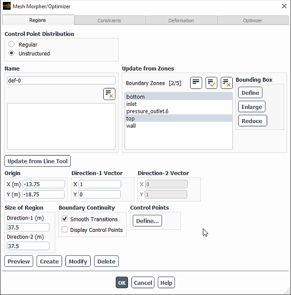
Define the region(s) of the domain where the mesh will be deformed in order to optimize the shape, by performing the following steps. Each deformation region will be defined as a “box”, that is, a rectangle for 2D cases and a rectangular hexahedron for 3D cases.
Important: It is recommended that you define each deformation region to be bigger than the area of interest, in order to maintain proper continuity between deforming and non-deforming regions.
In the Regions tab, enter a name for a deformation region in the text-entry box at the top of the Name group box.
You have the option of using the boundary zones to create a bounding box for the deformation region; this box can represent the final scope of the region, or it can act as a starting point that is further refined by manually editing the origin, direction vectors, and size of the region (as described in the steps that follow). Perform the following steps in the Update from Zones group box:
Select the zones from the Boundary Zones list that best represent the extents of the deformation region you would like to create.
Click the Define button in the Bounding Box group box to update the values in the Origin , Direction-1 Vector , Direction-2 Vector (for 3D cases), and Size of Region group boxes. Note that the bounding box will be previewed in green in the graphics window when you click any of the Bounding Box buttons.
You can increase or decrease the size of the bounding box by clicking the and buttons, respectively. Note that you have the option of setting the scaling factors associated with these buttons via the following text commands:
define→mesh-morpher-optimizer→region→scaling-enlargedefine→mesh-morpher-optimizer→region→scaling-reduce
You have the option of using the line tool (for 2D cases) or the plane tool (for 3D cases) to define the direction vectors of the deformation region; the values defined can represent the final components of the vectors, or they can act as a starting point that is further refined by manually editing the direction vectors (as described in the steps that follow). Set up the line tool or the plane tool (as described in Using the Line Tool and Using the Plane Tool, respectively), and then click the or button to update the values in the Direction-1 Vector and (for 3D cases) Direction-2 Vector group boxes.
Open the Line/Rake Surface Dialog Box or the Plane Surface Dialog Box to make the line or plane tool appear.
Define an origin for the deformation region by entering the Cartesian coordinates of a point in the X , Y, and (for 3D) Z number-entry boxes in the Origin group box. Note that as you enter values, you can view the resulting bounding box (in green) by clicking the button.
Define the first direction vector of the deformation region relative to the Origin coordinates, by entering values in the X, Y, and (for 3D) Z number-entry boxes in the Direction-1 Vector group box.
For 2D cases, Ansys Fluent will automatically define the second direction vector of the deformation region to be perpendicular to the Direction-1 Vector, and will display the components in the uneditable Direction-2 Vector group box.
For 3D cases, define the second direction vector of the deformation region relative to the Origin coordinates, by entering values in the X, Y , and Z number-entry boxes in the Direction-2 Vector group box. If the vector you define is not perpendicular to the Direction-1 Vector, Ansys Fluent will automatically redefine the second vector to be the projection of the Direction-2 Vector you entered onto a plane that is perpendicular to the Direction-1 Vector. Based on this definition, the Direction-2 Vector you define cannot be colinear with the Direction-1 Vector.
The third direction vector of the deformation region will be automatically defined as the cross product of the first and second direction vectors.
Define the overall dimensions of the deformation region by entering length values for Direction-1 , Direction-2, and (for 3D cases) Direction-3 in the Size of Region group box.
Create control points within the deformation region.
If you selected Regular for the Control Point Distribution, define the number of control points you want along each direction vector of the deformation region by entering values for Direction-1 , Direction-2, and (for 3D cases) Direction-3 in the Control Points group box. The total number of control points for the region will be the product of the numbers you enter. Increasing the number of control points allows you greater control of the deformation, but also increases the computational expense.
Important: When you define multiple deformation regions, you must ensure that all the deformation regions have the same total number of control points.
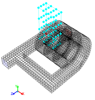
Save the settings you have created for the deformation region by clicking the Create button. The name of the deformation region will be added (and selected) in the selection list at the bottom of the Name group box, and the control points and bounding box of the deformation region will be displayed in blue in the graphics window (see Figure 48.39: Displaying the Control Points for a Regular Distribution). If you do not want the control points and bounding box displayed in the graphics window, you can deselect the item by clicking the button located above the right side of the Name selection list.
A new default name will be automatically entered in the text-entry box at the top of the Name group box, in preparation for any deformation regions you want to create in the future.
If you selected Unstructured for the Control Point Distribution, click the button to save the settings for the deformation region, as you need an existing region to be able to create control points. The name of the deformation region will be added (and selected) in the selection list at the bottom of the Name group box, and the bounding box will be displayed in blue in the graphics window (see Figure 48.41: Displaying the Control Points for an Unstructured Distribution). If at any point you do not want the bounding box displayed in the graphics window, you can deselect the item by clicking the button located above the right side of the Name selection list.
Next, examine the settings in the Boundary Continuity group box. By default, the mesh morpher/optimizer is set to provide smooth mesh transitions wherever the mesh intersects with the limits of the deformation region (that is, the sides of the bounding box). This is accomplished through the creation of stationary control points at those intersections; by default, these control points are hidden, though you can view them by enabling the Display Control Points option. If you would like to allow more abrupt mesh transitions at the boundaries of the region, you can disable the Smooth Transitions option.
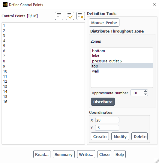
The next step is to create control points. Click the button in the Control Points group box to open the Define Control Points dialog box ( Figure 48.40: The Define Control Points Dialog Box).
Use the Define Control Points dialog box to create control points within the region. You have the following options:
Click the button and then probe (using the right mouse button, by default) within the deformation region. For 3D cases, if you probe on a displayed boundary, the control point will be located at that point on that boundary. Note that it may be helpful to revise what surfaces are displayed using the Mesh Display Dialog Box.
Make a selection from the Zones list, enter an Approximate Number of control points that you want on that zone, and click the button. This method uses Binary Space Partitioning (BSP) to agglomerate the cell faces of the zone within the bounding box based on the intended number of control points, and then a control point is assigned to the node that is closest to the centroid of each agglomeration. While this method is convenient when you want a large number of control points or want to morph entire boundary zones or surfaces, there are some limitations to BSP: the number of control points may exceed the value you enter, and the control points will not be as evenly distributed on curved surfaces when compared to flat surfaces.
Enter X, Y , and Z coordinates and click the button. This method allows you to locate a control point directly on a mesh node, if you have first obtained the vertex position (which can be displayed in the console if you select long description from the Probe drop-down list in the View tab (Mouse group box) and then probe near the node with the mouse).
If you have previously generated an ASCII text file that contains control point definitions, you can read it by clicking and using the dialog box that opens. Using a text file can be helpful when you have a large number of points. It is not necessary to create the text file from scratch, as you can create a simplified text file with sample data using the button, and then define the bulk of the control point locations using a spreadsheet program. See Mesh Morpher/Optimizer File Formats for details about the format of the text file.
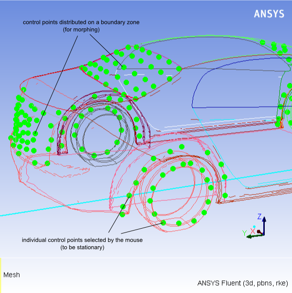
The control points will be displayed in green in the graphics window, and will turn red when selected in the Control Points selection list. When a control point is selected, you also have the ability to it, or enter new coordinates and it.
When adding control points, remember that it may be helpful to locate them not only in areas that you want to deform, but also on features in the deformation region that you want to preserve (as you can make nodes stationary by applying a parameter value of zero). When you are done adding control points, click to close the Define Control Points dialog box.
A new default name will be automatically entered in the text-entry box at the top of the Name group box, in preparation for any deformation regions you want to create in the future.
Create any additional deformation regions as necessary by repeating steps 5.a.–h.
Important: Overlapping deformation regions are not supported.
If you need to modify a deformation region at any point, select it in the Name selection list, revise the appropriate settings, and click the button. The updated control points and bounding box will be displayed in the graphics window.
Important: When modifying an existing deformation region, be sure to click rather than . If you click , you will not modify the deformation region, but will instead create a new one with the modified settings.
If you need to delete a deformation region at any point, select it in the Name selection list and click the button.
You have the option of defining constraints on the boundary zones, in order to limit the freedom of particular zones that fall within the deformation region(s) during the morphing of the mesh. The following options are available:
unconstrained
This option specifies that the boundary zone is completely free to be deformed according to the assigned parameters. By default, all wall zones are unconstrained.
fixed
This option specifies that the boundary zone is fixed and will not be deformed. None of the zones are fixed by default.
Important: If you specify one or more fixed boundary zones in a deformation region, you must ensure that there is at least one unconstrained boundary zone in the region as well.
passive
This option specifies that the nodes of the boundary zone are partially constrained to varying degrees, based on their proximity to adjacent boundary zones that are fixed. The nodes in a passive boundary zone behave in a similar manner to the interior mesh nodes, in order to ensure that there is a smooth transition between fixed and unconstrained boundary zones. By default, all boundary zones that are not walls (for example, inlets, outlets, symmetry, and periodic boundaries) are passive.
To define the constraints on the boundary zones, perform the following steps.
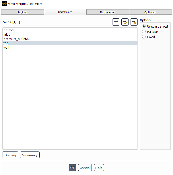
Click the Constraints tab (Figure 48.42: The Constraints Tab of the Mesh Morpher/Optimizer Dialog Box).
To revise the default constraints on the boundary zones, select the zone name(s) from the Zones selection list in the Constraints group box, and then select either Unconstrained, Passive , or Fixed from the Option list.
Click if you want view the boundary zones selected from the Zones selection list, in order to verify the zones for which you are defining constraints.
Click if you would like to print a list in the console that summarizes the constraint definitions for all of the boundary zones.
Begin the deformation definition by defining the parameters.
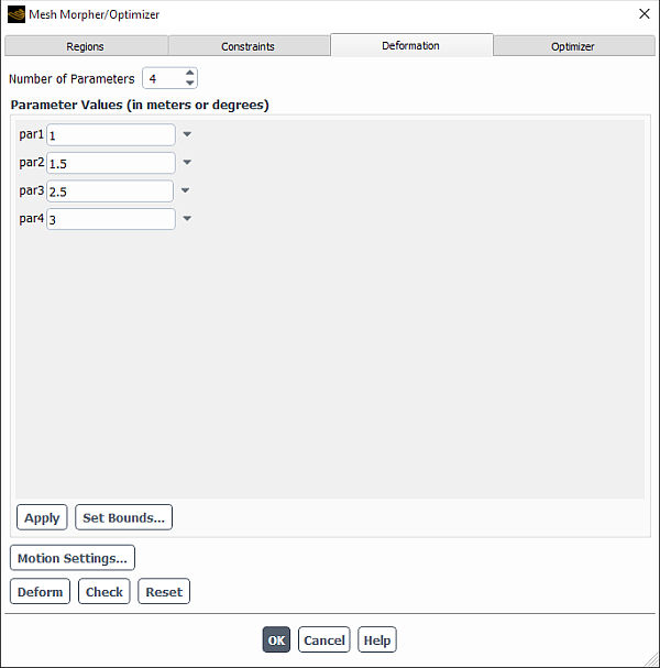
Click the Deformation tab (Figure 48.43: The Deformation Tab of the Mesh Morpher/Optimizer Dialog Box).
Enter the Number of Parameters that will be used to define the deformation. This number may be as low as the maximum number of parameters you will define on a single control point, or as high as the total number of parameters you will set on all of the control points combined.
If you want to manually specify the deformation or use Design Exploration in Ansys Workbench to explore multiple deformation scenarios (rather than using the built-in optimizers), define the parameter fields in the Parameter Values group box. Note that these fields are only available when none or workbench is selected from the Optimizer drop-down list in the Optimizer tab. The value of the parameter defines a magnitude that will then be used along with other direction settings to define motions that produce an overall displacement for a given control point. The value will specify a length in meters for translations and radial motions, and will specify an angle in degrees for rotations; the units here will be used regardless of what units you are using in the case.
For each parameter you have the following options:
Enter a constant numeric value. Note that having a parameter with a value of zero allows you to make a control point stationary.
Use the drop-down menu to define the parameter through an expression or input parameter (for example, as part of a parametric study managed by Workbench); for details, see Directly Applied Expressions or Creating a New Parameter, respectively.
When you have finished defining the parameter fields, click the button in the Parameter Values group box to save the definitions.
You have the option of limiting how much each parameter is allowed to deform by defining strict minimum and maximum values. This can be useful when you need to keep the parameters within a certain tolerance of the initial design, or when you know in advance that certain designs are impractical. While this option is typically used with the built-in optimizers, it is available for manual deformation, so that you can visualize the effects of the bounds and set them interactively. Note that this option is not available when workbench is selected from the Optimizer drop-down list in the Optimizer tab.
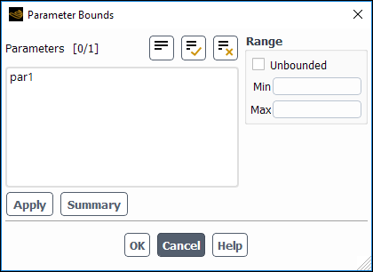
Click the button in the Parameter Values group box to open the Parameter Bounds dialog box (Figure 48.44: The Parameter Bounds Dialog Box).
Select the parameters you want to limit from the Parameters selection list, disable the Unbounded option in the Range group box, and then enter appropriate values for Min and Max.
At any point you can click the button to save your bounds, and you can click the Summary button to display a summary of the saved bounds in the console. When all of the parameter bounds are defined to your satisfaction, click the button to close the Parameter Bounds dialog box.
If you selected Regular for the Control Point Distribution in the Regions tab, perform the following steps. You will define motion settings for the control points by selecting parameters (which you defined previously) and specifying the translation direction, thus completing the deformation definition.
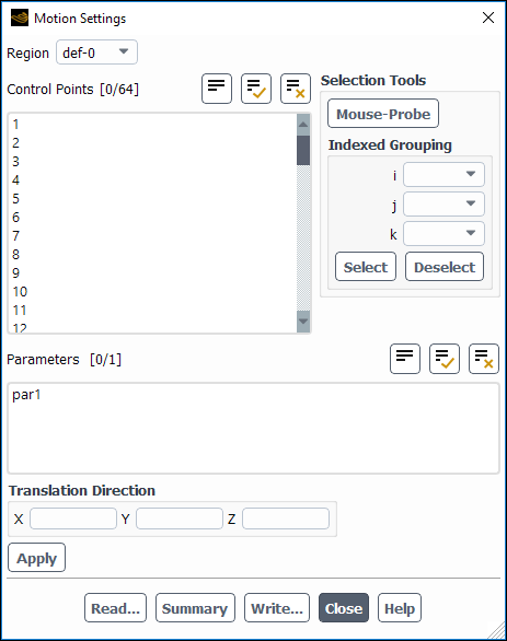
Click the button in the Deformation tab to open the Motion Settings dialog box (Figure 48.45: The Motion Settings Dialog Box for a Regular Distribution).
(optional) If you have previously generated an ASCII text file that contains motion settings, you can read it by clicking at the bottom of the Motion Settings dialog box and using the dialog box that opens; otherwise, you should proceed to steps 8.c.–8.j. and define the settings using the other controls in the Motion Settings dialog box.
Using a text file can be helpful when you have a large number of motion settings. It is not necessary to create the text file from scratch, as you can create a simplified text file with sample values using the button (as described in step 8.k.), and then add the bulk of the motion settings using a spreadsheet program. See Mesh Morpher/Optimizer File Formats for details about the format of the text file.
Important: Immediately after you read a text file, the Motion Settings dialog box will not display the applied settings. To begin viewing the applied settings, make a selection from the Region, Control Points, and Parameters lists, and the associated Translation Direction will be displayed.
You can then edit the motion settings as necessary (in a manner similar to steps 8.c.–8.g.) and/or proceed to step 8.m.
Make a selection from the Region drop-down list in the Motion Settings dialog box.
Specify the control points in the current Region to which you want to assign the same motion settings (that is, the same combination of parameters and direction). You can specify these control points using one or more of the following methods:
Select the ID numbers from the Control Points selection list. The selected control points will be highlighted in the graphics window.
Click the button in the Selection Tools group box and then click the control points in the graphics window with the mouse-probe button (which is the right mouse button, by default). To deselect, select a highlighted control point with the mouse-probe button. As you select the control points, they will also be selected in the Control Points selection list.
Use the Indexed Grouping group box to select the control points based on their assigned indices. Each control point has i , j, and (for 3D cases) k index numbers, each of which denote its place in the sequence (starting at the origin of the region) of control points along the direction-1, direction-2, and direction-3 vectors, respectively (as defined in the Regions tab of the Mesh Morpher/Optimizer dialog box). You can make selections from the index drop-down lists, and then click the button. In a similar way you can deselect control points using the button. As you select the control points, they will also be selected in the Control Points selection list and highlighted in the graphics window.
For example, consider the case of a 3D region: if you select 2 from the k drop-down list, the control points in the second plane perpendicular to the direction-3 vector (that is, the direction-1–direction-2 plane) will be selected. If you select 1 from both the i and j drop-down lists, the line of control points at the intersection of the first planes perpendicular to the direction-1 and direction-2 vectors will be selected. Making selections from all three drop-down lists will select a single control point.
Make selections from the Parameters selection list, in order to specify those you want to assign (along with a translation direction) to the selected Control Points. Note that the values associated with these parameters (as displayed in the Parameter Values group box in the Deformation tab of the Mesh Morpher/Optimizer dialog box) are irrelevant if you plan to use the built-in optimizers.
Define the Translation Direction that will be associated with the selected Parameters by entering values for the X, Y, and (for 3D cases) Z directions. Note that you do not need to define a unit vector.
If you use a built-in optimizer, these values will provide the direction of the displacement of the control point and the optimizer will determine the overall magnitude of displacement. Alternatively, if you specify the deformation manually or using Design Exploration, the values you enter in the Translation Direction group box will be multiplied with the values of the Parameters to define the displacement applied to the control points.
Click the button to save the motion settings.
If you want to apply another set of motion settings to the selected Control Points, repeat steps 8.e.–8.g. for each additional combination of parameters and direction.
Repeat steps 8.d.–8.h. for each additional set of control points in the current Region to which you want to assign motion settings.
Repeat steps 8.c.–8.i. for each additional region in which you want to apply deformation parameters to control points.
If you want to save all of the settings you specified in the Motion Settings dialog box as an ASCII text file, click and specify a name in the dialog box that opens. You can edit the motion settings in this text file using a spreadsheet program, and then read it in this or a separate case file, as described in step 8.b.
You can display a summary of the motion settings in the console by clicking the button.
Click to close the Motion Settings dialog box.
If you selected Unstructured for the Control Point Distribution in the Regions tab, perform the following steps. You will define one or more motions—which consist of a parameter (defined previously), direction settings, and the affected control points—and thus complete the deformation definition.
Important: When a single control point is associated with multiple motions, note that the resultant displacement for each individual motion will be calculated from the original position, and then the displacements will be summed. This means that the order in which the motions are created will have no effect on the final location of the control point.
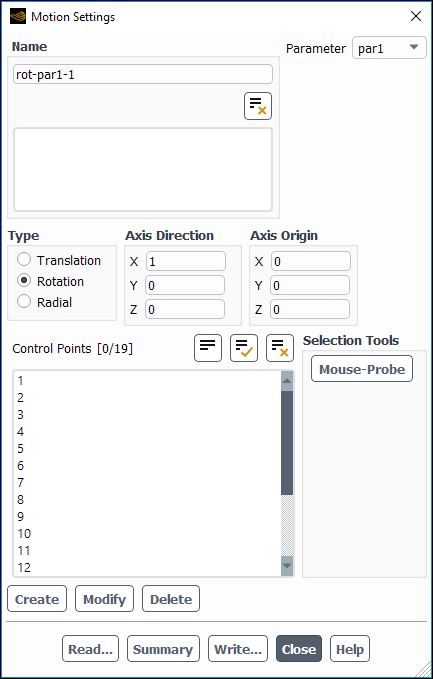
Click the button in the Deformation tab to open the Motion Settings dialog box (Figure 48.46: The Motion Settings Dialog Box for an Unstructured Distribution).
(optional) If you have previously generated an ASCII text file that contains motion definitions, you can read it by clicking at the bottom of the Motion Settings dialog box and using the dialog box that opens; otherwise, you should proceed to steps 9.c.–9.k. and define the settings using the other controls in the Motion Settings dialog box.
Using a text file can be helpful when you have a large number of motions. It is not necessary to create the text file from scratch, as you can create a simplified text file with sample values using the button (as described in step 9.l.), and then add the bulk of the motion definitions using a spreadsheet program. See Mesh Morpher/Optimizer File Formats for details about the format of the text file.
You can then either add additional motions (in a manner similar to steps 9c.–9.h.) or modify / delete an existing motion (as described in steps 9.i. and 9.j.). When the settings are finalized, you can proceed to step 9.k.
To begin defining a new motion, make a selection from the Parameter drop-down list.
Make a selection from the Type list, to indicate the type of motion you would like to define. You can specify that a group of control points undergoes a Translation, a Rotation about a point (for 2D) or an axis (for 3D), or a Radial motion about a point (for 2D) or an axis (for 3D).
Define the motion by entering X , Y, and (for 3D cases) Z values for the following: the Direction used for translations; or the Axis Origin and (for 3D cases) Axis Direction used for rotations and radial motions. For Direction or Axis Direction, note that you do not need to define unit vectors.
If you use a built-in optimizer, the values you enter will define the direction of the displacement of the control point and the optimizer will determine the overall magnitude of displacement. Alternatively, if you specify the deformation manually or using Design Exploration, the magnitude will be the value of the Parameter ; translation is a special case, in which the values you enter in the Direction group box are multiplied with the value of the Parameter to define the displacement applied to the control points.
Select the control points to which you want to assign the selected motion. You can either select them in the Control Points list, or click the button and click the control points in the graphics window using the mouse-probe button (which is the right mouse button, by default).
A default name will be generated in the top field of the Name group box, based on the Type and Parameter of the motion. You can edit this text to make it more descriptive, as necessary.
Click to create the motion. The name will be added to the selection list in the Name group box.
Repeat steps 9.c.–9.g. for each additional motion that you would like to create.
If you need to modify a motion at any point, select it in the lower selection list in the Name group box, revise the appropriate settings, and click the button.
Important: When modifying an existing motion, be sure to click rather than . If you click , you will not modify the motion, but will instead create a new one with the modified settings.
If you need to delete a deformation region at any point, select it in the lower selection list in the Name group box and click the button.
You can display a summary of the motion definitions in the console by clicking the button.
If you want to save all of the settings you specified in the Motion Settings dialog box as an ASCII text file, click and specify a name in the dialog box that opens. You can edit the motion settings in this text file using a spreadsheet program, and then read it in this or a separate case file, as described in step 9.b.
If you want to manually specify the deformation (that is, none is selected from the Optimizer drop-down list in the Optimizer tab of the Mesh Morpher/Optimizer dialog box), perform the following steps:
Click the button to apply the current settings (in the Parameter Values group box and Motion Settings dialog box) and to display the deformed mesh in the graphics window. The Deform button allows you to manually specify the deformation.
You can click the button to print out a mesh check report in the console for the currently displayed mesh. The mesh check report is the same as that produced by the Check button in the General task page, as described in Mesh Check Report.
Important: If you save parameter settings but do not click the button, the mesh check report will not account for the mesh that is produced from those settings.
Click the button if you want to revert to the original mesh without the deformations that result from the button.
If you plan to use the built-in optimizers, you should decide whether you want to disable the general mesh check that is performed by default immediately after the mesh is deformed in every design stage. The mesh check that is performed is the same as that initiated by the Check button in the General task page (see Checking the Mesh for details). If any errors are discovered, the mesh is rejected and the next design stage is attempted.
Disabling the general mesh check allows you to repair the mesh, so that an accurate solution can be calculated for it. Note that you can set up the mesh repair by entering the appropriate text commands (as described in Repairing Meshes) in the Initial Commands text-entry box in the Optimizer tab.
You can disable the general mesh check by using the following text command:
define→mesh-morpher-optimizer→optimizer-parameters→disable-mesh-checkIf you want to use the built-in optimizers, define the optimizer settings and initiate the optimization process.
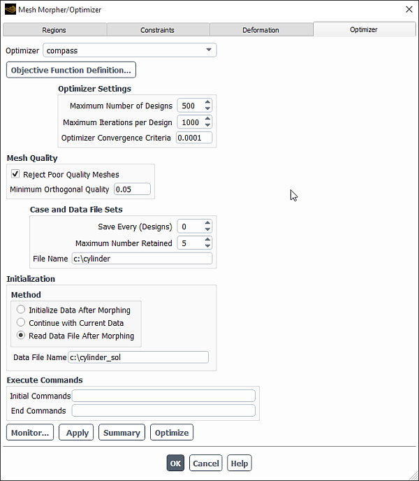
Click the Optimizer tab (Figure 48.47: The Optimizer Tab of the Mesh Morpher/Optimizer Dialog Box).
Select an optimizer from the Optimizer drop-down list. The available optimizers are not based on gradients, and include the following: compass , newuoa, powell , rosenbrock, simplex, and torczon. For more information about how these optimizers function, see Optimizers .
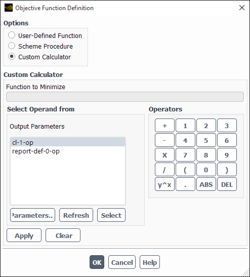
Click the button to open the Objective Function Definition dialog box (Figure 48.48: The Objective Function Definition Dialog Box).
Make a selection in the Options group box to specify whether the objective function that will be minimized during the optimization process is a User-Defined Function, a Scheme Procedure, or a customized function of output parameters as defined by the Custom Calculator. Your selection should correspond with the actions you took in step 2.
If you selected Custom Calculator in the previous step, define the objective function via the GUI controls in the Custom Calculator group box. As you click the buttons in this group box, text and symbols will appear in the Function to Minimize text box. You cannot edit the contents of this box directly; if you want to delete part or all of the function, use the or button, respectively.
You can include output parameters in the definition of the function by making a selection from the Output Parameters list and clicking . If you want to add a new output parameter to the selection list or check the definition of an existing one, you can click the button and use the Parameters dialog box (as described in Creating Output Parameters); be sure to click the button when you return to the Objective Function Definition dialog box, so that the Output Parameters list is updated. You can also use Operators to manipulate the output parameters in the function.
You can click the button at any point to save your function. When it is fully defined, click the button to save your settings and close the Objective Function Definition dialog box.
Define the settings in the Optimizer Settings group box.
Enter a value for Maximum Number of Designs, to specify the maximum number of design stages the optimizer will undergo to reach the specified objective function. Note that this number is not the number displayed in the console during the optimization process. Each optimizer undergoes a certain number of design modifications (called “runs”) before it converges to a design for a particular design stage. The
Runnumber displayed in the console refers to the actual design modifications (including the inner loop) irrespective of the optimizer, whereas the Maximum Number of Designs value is the maximum number of converged designs provided by the optimizer.Enter the Maximum Iterations per Design , to specify the maximum number of iterations Ansys Fluent performs for each design change.
Enter a number for Optimizer Convergence Criteria, to specify the convergence criteria for the optimizer.
If you selected the newuoa optimizer, enter a number for the Initial Parameter Variation to specify how much the parameters will be allowed to vary during the initial calculations. This value is not intended to define a strict minimum / maximum for the parameters (as is defined by the bounds specified using the Parameter Bounds dialog box), but should only be large enough to allow the optimizer to capture the minima. A better estimation (that is, a smaller value) allows the optimizer to reach convergence faster.
By default, the orthogonal quality (as defined in Mesh Quality) of the initial and every subsequent mesh is computed, before the related solution calculation is initiated. If the orthogonal quality for any cell is less than a specified value, the mesh is rejected and Fluent proceeds to the next design stage (therefore helping to ensure that your solution accuracy is not compromised by poor quality meshes). These actions are governed by the settings in the Mesh Quality group box.
If you do not want the meshes rejected based on their orthogonal quality, you can disable the Reject Poor Quality Meshes option; otherwise, specify the minimum orthogonal quality that must be maintained by every cell by entering a value from
0–1(where0represents the worst quality) for Minimum Orthogonal Quality. When determining an appropriate minimum value, you can check the orthogonal quality of the initial mesh (by using the button in the General task page) and then select a value that is sufficiently lower, so as not to reject a majority of the meshes generated during the optimization process.You have the option of saving intermediate case and data files during the optimization run, so that you can restart an interrupted solution in the same or a different Fluent session without increasing the overall number of design iterations needed to reach convergence. To enable the saving of such intermediate files, define the settings in the Case and Data File Set group box.
Specify the frequency (in number of design iterations) that you want the intermediate case and data files saved by entering a value for Save Every. The default value is 0, which specifies that no intermediate files will be saved. Note that if you selected the newuoa optimizer, the frequency at which files are saved may not exactly correspond to the number you enter, but should be reasonably close.
Specify the maximum number of intermediate files sets you want to retain by entering a value for Maximum Number Retained. After the maximum limit of file sets has been saved, Ansys Fluent begins overwriting the earliest existing intermediate file set. Lower values should be used if you have limited disk space or you are concerned about saving unnecessary files.
Specify a root name for the intermediate files in the File Name text box. When the files are saved, the design iteration will be appended to this root name to indicate the point at which it was saved during the optimization run. An extension will also be automatically added to the root name (
.cas.h5or.dat.h5, by default). You can include a folder path in the filename if you want the files saved outside of the working folder.
Specify how the solution variables should be treated after the mesh is deformed by making a selection from the Method list in the Initialization group box:
Select Initialize Data After Morphing to specify that the solution variables should be initialized to the values specified in the Solution Initialization task page after deformation.
Select Continue with Current Data to specify that the solution variables remain the values obtained in the previous design stage. This selection will reduce the number of iterations needed to reach convergence compared to the Initialize Data After Morphing selection. Note that if the solver diverges during an intermediate design stage, the solution variables will be initialized and the solution will be attempted again.
Select Read Data File After Morphing to specify that the solution variables are set to the values obtained from the data file specified in the Data File Name text-entry box. This selection will reduce the number of iterations needed to reach convergence compared to Initialize Data After Morphing selection or (in cases where the solution diverges for an intermediate design stage) the Continue with Current Data selection. Note that this selection is not available when newuoa is selected from the Optimizer drop-down list.
If you did not select the newuoa optimizer, you have the option of specifying commands that will be executed during the optimization runs of the mesh morpher/optimizer, via the text-entry boxes in the Execute Commands group box. A command can be a text command or the name of a command macro you have defined (or will define), as described in Defining Macros. You can also enter a series of text commands and/or macros, as long as they are separated by a semi-colon (
;).During optimization runs, deformation occurs as part of every design iteration. You decide the specific point during the design iteration that the command is executed:
If you want a command to be executed after the design has been modified, but before Ansys Fluent has started to run the calculation for that design stage, enter the command in the Initial Commands text-entry box. There are no restrictions on the commands that can be entered: you can enter commands that read saved data, perform FMG initialization, execute an entirely independent on-demand UDF, or even call a Scheme routine.
If you want a command to be executed after the solution has run and converged for a design stage, enter the command in the End Commands text-entry box. There are no restrictions on the commands that can be entered. Examples are commands for postprocessing solution variables, monitoring contours and vectors of different variables, taking snapshots of each design change, and so on, at every design stage.
Important: If the command to be executed involves saving a file, see Saving Files During the Calculation for important general information.
As noted in Automatic Numbering of Files, the special character,
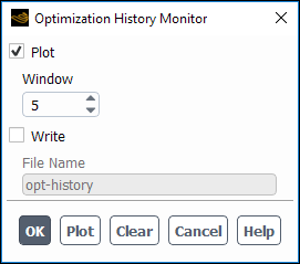
%i, can be used to create unique filenames by including the iteration number. However, by default, the solution will be initialized after each mesh deformation and the iteration count restarted. Therefore, the resulting filename cannot be used to identify which design stage produced it (that is, the first design stage may converge at 50 iterations, and then the second design stage may converge at 43 iterations). The time that the file was created is a better way to identify where in the series of design stages the file was generated. In addition, some files may be overwritten if two design stages converge in the same number of iterations. Alternatively, if you have selected Continue with Current Data under Initialization when setting up the optimizer, then the iteration count will not reset and no duplicate filenames will occur.If you did not select the newuoa optimizer, you can plot and/or record the optimization history (that is, how the value of the objective function varies with each design stage). Click the button to open the Optimization History Monitor dialog box (Figure 48.49: The Optimization History Monitor Dialog Box) and perform the steps that follow.
Enable the option if you want to display a plot of the optimization history, which will automatically be plotted in an appropriate graphics window.
Enable the Write option if you want to save the optimization history data in a file, and specify the File Name.
Note that you can display a plot of the optimization history data generated during the last calculation, even if the Plot or the Write options were not enabled during the calculation, as long as you have not discarded the data using the button. Simply click the button and the plot will be displayed in the active graphics window.
Click the button to save your optimizer settings.
Click the button to display a summary of the mesh morpher/optimizer settings in the console.
Click the button to initiate the optimization process. Information about each run (that is, each design modification) that is generated as part of the production of a design stage will be displayed in the console, and the deformed mesh for each run will be updated in the graphics window.
If you set up the saving of intermediate case and data files in step 12.f and your solution is interrupted during the optimization run, you can restart the calculation using the latest intermediate files. Note that you should not revise the deformation regions or constraint settings for the restarted mesh.
If you want to use Design Exploration in Ansys Workbench to explore multiple deformation scenarios, define the optimizer settings.
Click the Optimizer tab (Figure 48.47: The Optimizer Tab of the Mesh Morpher/Optimizer Dialog Box).
Select workbench from the Optimizer drop-down list. Note that workbench is only available if you have launched your Ansys Fluent session from Ansys Workbench.
If necessary, revise the default settings in the Mesh Quality group box, as described in step 12.e. Note that the design point associated with a poor quality mesh will not be updated in Workbench.
Click to close the Mesh Morpher/Optimization dialog box.
If you want to use Design Exploration in Ansys Workbench to explore multiple deformation scenarios, save your case file and close your Ansys Fluent session. You can then proceed to Ansys Workbench and define the design points that will provide the multiple values for the input parameters you created / assigned in step 7.c. For more information about using design points to explore Ansys Fluent results, see Working With Input and Output Parameters in Workbench in the Ansys Fluent in Workbench User's Guide.
If you manually deformed the mesh or used the built-in optimizers, run your case file with the deformed mesh.
If you want to rerun a case file in which the mesh has been deformed by the Optimize button in the Optimizer tab, you should not revise the deformation regions or constraint settings for the deformed mesh.