


Cell zones consist of fluids and solids. Porous zones and 3D fans in Ansys Fluent are treated as fluid zones. A detailed description of the various cell zones is given in the sections that follow.
A fluid zone is a group of cells for which all active equations are solved. The only required input for a fluid zone is the type of fluid material. You must indicate which material the fluid zone contains so that the appropriate material properties will be used.
Important: If you are modeling multiphase flow, you will not specify the materials here; you will choose the phase material when you define the phases, as described in Defining the Phases for the VOF Model.
Important: If you are modeling species transport and/or combustion, you can specify the material as either a mixture or a fluid. The mixture material has to be the same as that specified in the Species Model dialog box when you enable the model. The fluid zones, being of different material types, must not be contiguous.
Optional inputs allow you to set sources or fixed values of mass, momentum, heat (temperature), turbulence, species, and other
scalar quantities. You can also define motion for the fluid zone. If there are rotationally periodic boundaries adjacent to the fluid
zone, you must specify the rotation axis. If you are modeling turbulence using one of the  -
-  models, the
  -
-  model, or the Spalart-Allmaras model, you can choose to define the fluid zone as a laminar flow region. If you
are modeling radiation using the DO model, you can specify whether or not the fluid participates in radiation.
model, or the Spalart-Allmaras model, you can choose to define the fluid zone as a laminar flow region. If you
are modeling radiation using the DO model, you can specify whether or not the fluid participates in radiation.
Warning: In general, disabling Participates in Radiation for fluid zones is not recommended, as it can produce erroneous results. There are rare cases when it is acceptable: for example, if the domain contains multiple fluid zones, disabling this option for zones where radiation is negligible may save computational time without affecting the results.
Important: For information about porous zones and 3D fan zones, see Porous Media Conditions and 3D Fan Zones, respectively.
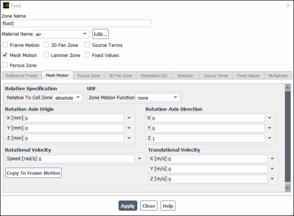
You will set all fluid conditions in the Fluid Dialog Box (Figure 7.11: The Fluid Dialog Box), which is accessed from the Cell Zone Conditions task page (as described in Setting Cell Zone and Boundary Conditions).
To define the material contained in the fluid zone, select the appropriate item in the Material Name drop-down list. This list will contain all fluid materials database) in the Create/Edit Materials Dialog Box. If you want to check or modify the properties of the selected material, you can click to open the Edit Material dialog box; this dialog box contains just the properties of the selected material, not the full contents of the standard Create/Edit Materials dialog box.
Important: If you are modeling species transport or multiphase flow, the Material Name list will not appear in the Fluid dialog box. For species calculations, the mixture material for all fluid zones will be the material you specified in the Species Model Dialog Box. For multiphase flows, the materials are specified when you define the phases, as described in Defining the Phases for the VOF Model.
If you want to define a source of heat, mass, momentum, turbulence, species, or other scalar quantity within the fluid zone, you can do so by enabling the Source Terms option. See Defining Mass, Momentum, Energy, and Other Sources for details.
If you want to fix the value of one or more variables in the fluid zone, rather than computing them during the calculation, you can do so by enabling the Fixed Values option. See Fixing the Values of Variables for details.
When you are calculating a turbulent flow, it is possible to “turn off” turbulence modeling in a specific fluid zone. To disable turbulence modeling, turn on the Laminar Zone option in the Fluid dialog box. This is useful if you know that the flow in a certain region is laminar. For example, if you know the location of the transition point on an airfoil, you can create a laminar/turbulent transition boundary where the laminar cell zone borders the turbulent cell zone. This feature allows you to model turbulent transition on the airfoil.
By default, the Laminar Zone option will set the turbulent viscosity,  , to zero and disable turbulence production in the fluid zone. Turbulent quantities will still be transported
through the zone, but effects on fluid mixing and momentum will be ignored. If you want to keep the turbulent viscosity, you
can do so using the text command
, to zero and disable turbulence production in the fluid zone. Turbulent quantities will still be transported
through the zone, but effects on fluid mixing and momentum will be ignored. If you want to keep the turbulent viscosity, you
can do so using the text command define/ boundary-conditions/fluid. You will
be asked if you want to Set Turbulent Viscosity to zero within laminar zone?. If your response is
no, Ansys Fluent will set the production term in the turbulence transport equation to zero, but will
retain a nonzero  .
.
Disabling turbulence modeling in a fluid zone can be applied to all the turbulence models except the Large Eddy Simulation (LES) model.
If you are modeling species transport with reactions, you can enable a reaction mechanism in a fluid zone by turning on the Reaction option and selecting an available mechanism from the Reaction Mechanism drop-down list. See Defining Zone-Based Reaction Mechanisms for more information about defining reaction mechanisms.
If there are rotationally periodic boundaries adjacent to the fluid zone or if the zone is rotating, either the mesh or its reference frame, you must specify the rotation axis. To define the axis for a moving reference frame problem, set the Rotation-Axis Direction and Rotation-Axis Origin under the Reference Frame tab. To define the axis for a moving mesh problem, set the Rotation-Axis Direction and Rotation-Axis Origin under the Mesh Motion tab.
Note: If a frame motion and a mesh motion are specified at the same zone and this zone has rotationally periodic boundaries adjacent to it, then both axes have to be coaxial. Otherwise, the periodicity assumption is not valid and you will receive a warning message. In addition, the mesh check will fail.
The cell zone axis is independent of the axis of rotation used by any adjacent wall zones or any other cell zones. For 3D
problems, the axis of rotation is the vector from the Rotation-Axis Origin in the direction of the vector
given by your Rotation-Axis Direction inputs for the frame of reference and the mesh motion. For 2D
non-axisymmetric problems, you will specify only the Rotation-Axis Origin; the axis of rotation is the
 -direction vector passing through the specified point. (The
  direction is normal to the plane of your geometry so that rotation occurs in the plane.) For 2D axisymmetric
problems, you will not define the axis: the rotation will always be about the
direction is normal to the plane of your geometry so that rotation occurs in the plane.) For 2D axisymmetric
problems, you will not define the axis: the rotation will always be about the  axis, with the origin at (0,0).
To define zone motion for a moving reference frame (MRF), enable the Frame Motion option in the Fluid dialog box. Set the appropriate parameters in the expanded portion of the dialog box, under the Reference Frame tab. For further details on such simulations, see Modeling Flows with Moving Reference Frames.
To define zone motion for a moving (sliding) mesh, enable the Mesh Motion option in the Fluid dialog box. Set the appropriate parameters in the expanded portion of the dialog box, under the Mesh Motion tab. See Setting Up the Sliding Mesh Problem for details.
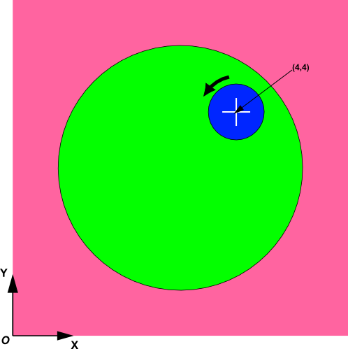
For cases that do not contain zones with motion specified in a relative frame to another zone, select absolute from the Relative To Cell Zone drop-down list. Here, the velocity and rotation components are specified in an absolute reference frame, which is the default setting, as shown in Figure 7.12: Rotation Specified in the Absolute Reference Frame. If no moving zones are present in the simulation, then absolute will be the only available selection. See The Multiple Reference Frame Model for more information.
For cases where you have a moving zone specified relative to another moving zone, select the cell zone carrying the primary motion from the Relative To Cell Zone drop-down list under the Reference Frame tab or the Mesh Motion tab. Note that for such cases, Rotation-Axis Origin (Relative) will appear in the interface, signifying coordinates relative to the zone selected from the Relative To Cell Zone drop-down list.
Figure 7.13: Rotation Specified Relative to a Moving Zone illustrates that the rotational axis origin of the small rotating zone is
specified relative to the cell zone carrying the primary motion (having local coordinate system  ).
).
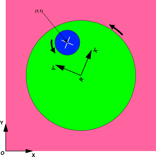
Note: The Relative To Cell Zone list will consist of all moving cell zones with an absolute motion specification (that is zones that are moving, but their motion is not relative to some other zone), excluding the current cell zone.
For problems that include linear, translational motion of the fluid zone, specify the Translational Velocity by setting the X, Y, and Z components under the Mesh Motion tab. For problems that include rotational motion, specify the rotational Speed under Rotational Velocity. The rotation axis is defined as described above. Note that the speed can be specified as a constant value or a transient profile. The transient profile may be in a file format, as described in Transient Cell Zone and Boundary Conditions, or a UDF macro (DEFINE_TRANSIENT_PROFILE). Specifying the individual velocities as either a profile or a UDF allows you to specify a single component of the frame motion individually. However, you can also specify the frame motion using a user-defined function. This may prove to be quite convenient if you are modeling a more complicated motion of the moving reference frame, where the hooking of many different user-defined functions or profiles can be cumbersome.
Important: If you need to switch between the MRF and moving mesh models, simply click the Copy To Mesh Motion
for zones with a moving frame of reference and Copy to Frame Motion for zones with moving meshes to
transfer motion variables, such as the axes, frame origin, and velocity components between the two models. The variables
used for the origin, axis, and velocity components, as well as for the UDF DEFINE_ZONE_MOTION
will be copied. This is particularly useful if you are doing a steady-state MRF simulation to obtain an initial solution
for a transient Moving Mesh simulation in a turbomachine.
Note that when a fluid zone undergoes normal zone motion relative to an adjacent solid zone, energy transfer at that boundary (that is, the total heat transfer rate) includes pressure work when the absolute velocity formulation is used. This pressure work is on the fluid side only, not on the solid side. For details on reporting the total heat transfer rate and/or pressure work rate, see Generating a Flux Report.
See Modeling Flows with Moving Reference Frames for details about modeling flows in moving reference frames. Details about
the frame motion UDF can be found in DEFINE_ZONE_MOTION in the Fluent Customization Manual.
If you are using the DO radiation model, you can specify whether or not the fluid zone participates in radiation using the Participates in Radiation option. See Defining Boundary Conditions for Radiation for details.
A “solid” zone is a group of cells for which no flow equations are solved: in a fluid simulation, only a heat conduction problem is solved; in an intrinsic fluid-structure interaction (FSI) simulation, displacement and stress tensor components are calculated. The material being treated as a solid may actually be a fluid, but it is assumed that no convection is taking place. The only required input for a solid zone is the type of solid material. You must indicate which material the solid zone contains so that the appropriate material properties will be used. Optional inputs allow you to set a volumetric heat generation rate (heat source) or a fixed value of temperature. You can also define motion for the solid zone. If there are rotationally periodic boundaries adjacent to the solid zone, you must specify the rotation axis. If you are modeling radiation using the DO model, you can specify whether or not the solid material participates in radiation.t.
Note that the solver will always visit the active equations, including flow and possibly turbulence equations, during solver iterations. This will happen even if all the cell zones existing in the domain are solid and there is no fluid zone in the domain. In order to improve the solver performance, you may want to deactivate the flow, and turbulence equations manually when there is only solid cell zones in the domain and fluid properties are not important.
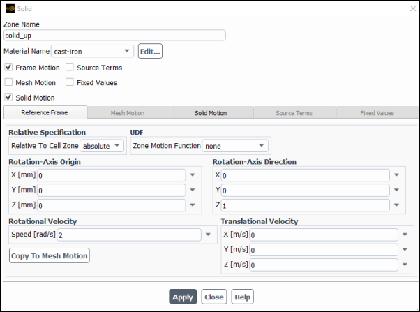
You will set all solid conditions in the Solid Dialog Box (Figure 7.14: The Solid Dialog Box), which is opened from the Cell Zone Conditions task page (as described in Setting Cell Zone and Boundary Conditions).
To define the material contained in the solid zone, select the appropriate item in the Material Name drop-down list. This list will contain all solid materials database) in the Create/Edit Materials Dialog Box. If you want to check or modify the properties of the selected material, you can click to open the Edit Material dialog box; this dialog box contains just the properties of the selected material, not the full contents of the standard Create/Edit Materials dialog box.
If you want to define a source of heat within the solid zone, you can do so by enabling the Source Terms option. See Defining Mass, Momentum, Energy, and Other Sources for details.
If you want to fix the value of temperature in the solid zone, rather than computing it during the calculation, you can do so by enabling the Fixed Values option. See Fixing the Values of Variables for details.
If there are rotationally periodic boundaries adjacent to the solid zone and you are not defining zone motion (as described in Defining Zone Motion), you must specify the cell zone axis by defining the Rotation-Axis Origin and Rotation-Axis Direction in the Reference Frame tab.
The cell zone axis is independent of the axis of rotation used by any adjacent wall zones or any other cell zones. For 3D
problems, the axis of rotation is the vector from the Rotation-Axis Origin in the direction of the vector
given by your Rotation-Axis Direction. For 2D non-axisymmetric problems, you will specify only the
Rotation-Axis Origin; the axis of rotation is the  -direction vector passing through the specified point. (The
  direction is normal to the plane of your geometry so that rotation occurs in the plane.) For 2D axisymmetric
problems, you will not define the axis: the rotation will always be about the
direction is normal to the plane of your geometry so that rotation occurs in the plane.) For 2D axisymmetric
problems, you will not define the axis: the rotation will always be about the  axis, with the origin at (0,0).
When defining motion for a solid zone, you have the following options:
You can enable the Frame Motion option for a moving reference frame (MRF) simulation only if the solid zone is not moving relative to an adjacent solid zone. Then define the settings in the Reference Frame tab. For further details on such simulations, see Modeling Flows with Moving Reference Frames.
You can enable the Solid Motion option if the solid zone is moving relative to an adjacent solid zone. Then define the settings in the Solid Motion tab.
To complete the setup for such a simulation, you must also define the velocity boundary conditions at coupled walls between the solid zone and any adjacent fluid zones; note that this is not necessary for the walls between the solid zone and any adjacent solid zones. For the fluid zone wall, you can choose to define the wall velocity based on the solid zone motion either as an absolute velocity or relative to the adjacent fluid zone. Details about these inputs are presented in Velocity Conditions for Moving Walls. When the energy equation is enabled, after you define the translational or rotational velocity for the solid in the Solid Mesh tab (as described in the steps that follow), you should enable the Boundary Advection option for the boundary walls through which heat is advected into or out of the domain to a significant degree; for details, see Boundary Advection for Solid Motion.
You can enable the Mesh Motion option for a moving (sliding) mesh, whether or not the solid zone is moving relative to an adjacent solid zone. Then define the settings in the Mesh Motion tab. For further details on such simulations, see Setting Up the Sliding Mesh Problem.
When defining the settings in the Reference Frame tab, Moving Mesh tab, and/or Solid Mesh tab, perform the following steps:
Make a selection from the Relative To Cell Zone drop-down list, in a manner similar to that described for fluid zones in Defining Zone Motion.
Define the Rotation-Axis Origin and Rotation-Axis Direction for the motion.
Note: If mesh motion is specified in the same zone as frame motion and/or solid motion and this zone has rotationally periodic boundaries adjacent to it, then both axes have to be coaxial. Otherwise, the periodicity assumption is not valid and you will receive a warning message. In addition, the mesh check will fail.
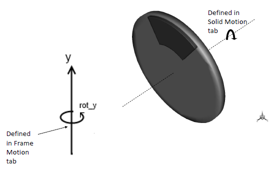
The only time it is possible to have separate axes defined is when combining solid motion with frame motion. For example, you could simulate an automotive disc brake assembly where a spinning rotor that is in contact with a brake pad is modeled using solid motion, while the rotation of the assembly about the vertical axis (due to input from the steering wheel) is modeled using frame motion (see Figure 7.19: Two solids in contact where one is stationary and the other is rotating. The rotational motion of the moving solid should be described in the Solid Motion tab. Both solids may also have rotation about the y-axis described in the Frame Motion tab. ).
The cell zone axis is independent of the axis used by any adjacent wall zones or any other cell zones. For 3D problems, the axis is the vector from the Rotation-Axis Origin in the direction of the vector given by your Rotation-Axis Direction. For 2D non-axisymmetric problems, you will specify only the Rotation-Axis Origin; the axis of rotation is the
-direction vector passing through the specified point. (The direction is normal to the plane of your geometry so that rotation occurs in the plane.) For 2D
axisymmetric problems, you will not define the axis: the rotation will always be about the axis, with the origin at (0,0).For problems that include linear, translational motion of the solid zone, specify the Translational Velocity by setting the X, Y, and Z components. For problems that include rotational motion, specify the rotational Speed under Rotational Velocity. The rotation axis is defined as described above. Note that the speed can be specified as a constant value or a transient profile. The transient profile may be in a file format, as described in Transient Cell Zone and Boundary Conditions, or a UDF macro (
DEFINE_TRANSIENT_PROFILE). Specifying the individual velocities as either a profile or a UDF allows you to specify a single component of the motion individually. However, you can also specify the motion using a user-defined function that uses the UDF macroDEFINE_ZONE_MOTION. This may prove to be quite convenient if you are modeling a more complicated motion, where the hooking of many different user-defined functions or profiles can be cumbersome.Important: Note that simultaneous translation and rotation can be modeled only if the rotation axis and the translation direction are the same (that is, the origin is fixed).
Note that if you decide to switch between the motion options for a solid zone, the user interface makes it easy to transfer motion variables, such as the axes, frame origin, and velocity components between the models:
If you need to switch from frame motion or solid motion to mesh motion, click the button. This is particularly useful if you are doing a steady-state MRF simulation to obtain an initial solution for a transient moving mesh simulation in a turbomachine.
If you need to switch from mesh motion to frame motion, simply click the button.
If you need to switch from frame motion to solid motion, enter the following text command:
mesh→modify-zones→convert-all-solid-mrf-to-solid-motionNote that this text command applies to all solid zones with frame motion enabled. It can be useful if you are updating a frame motion simulation that was set up in a previous release before solid motion was available.
For frame motion and/or solid motion, the velocity must be divergence-free, which requires that the specified motion be tangential to the boundaries. If the motion has a normal component, the solver cannot achieve energy conservation. The only exception, for which normal motion is permitted, is a coupled wall or mesh interface between two solid zones having the same material and motion. The solver will print a warning to the solver transcript the first time it encounters a solid velocity having a significant normal component at any other boundary type. The following examples illustrate valid solid zone motion definitions:

Figure 7.16: Rotating solid zone separated from another fluid or solid zone separated by a surface of revolution.
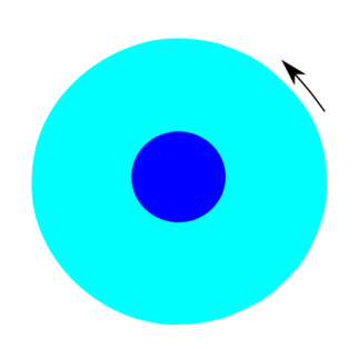
Figure 7.17: Multiple rotating solid zones having the same material and motion specifications, separated by mesh interfaces or coupled walls.
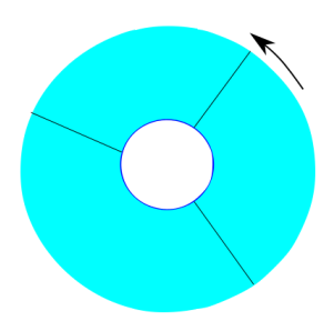
Figure 7.18: Two solids in contact where one is stationary and the other is moving with translational motion. The translational motion of the moving solid should be described in the Solid Motion tab.
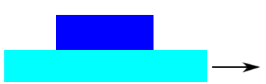
Figure 7.19: Two solids in contact where one is stationary and the other is rotating. The rotational motion of the moving solid should be described in the Solid Motion tab. Both solids may also have rotation about the y-axis described in the Frame Motion tab.
The following examples illustrate invalid frame motion or solid motion definitions for solid zones:
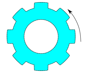
Figure 7.21: Two solids in contact with some squish. At the contact, the rotational motion has some normal component, so the solver will not achieve global energy conservation. However, the temperature field might still be acceptable for engineering purposes.
Limitations:
The effects of motion on the solid zone are applied only to the energy equation and the structural model calculations. User-defined scalars do not include the effects of motion.
Motion through a boundary zone adjacent to the solid zone is not permitted, though you can define a wall boundary with specified temperature condition; that is, there is no support for a 'solid inlet' or 'solid outlet'.
The Solid Motion option must not be enabled in a cell zone that has dynamic smoothing and/or layering enabled.
If you are using the DO radiation model, you can specify whether or not the solid material participates in radiation using the Participates in Radiation option. See Defining Boundary Conditions for Radiation for details.
The porous media model can be used for a wide variety of single phase and multiphase problems, including flow through packed beds, filter papers, perforated plates, flow distributors, and tube banks. When you use this model, you define a cell zone in which the porous media model is applied and the pressure loss in the flow is determined via your inputs as described in Momentum Equations for Porous Media. Heat transfer through the medium can also be represented, with or without the assumption of thermal equilibrium between the medium and the fluid flow (as described in Treatment of the Energy Equation in Porous Media).
A 1D simplification of the porous media model, termed the “porous jump,” can be used to model a thin membrane with known velocity/pressure-drop characteristics. The porous jump model is applied to a face zone, not to a cell zone, and should be used (instead of the full porous media model) whenever possible because it is more robust and yields better convergence. See Porous Jump Boundary Conditions for details.
The porous media model incorporates an empirically determined flow resistance in a region of your model defined as “porous”. In essence, the porous media model adds a momentum sink in the governing momentum equations. Consequently, the following modeling assumptions and limitations should be readily recognized:
Since the volume blockage that is physically present is not represented in the model, by default Ansys Fluent uses and reports a superficial velocity inside the porous medium, based on the volumetric flow rate, to ensure continuity of the velocity vectors across the porous medium interface. This superficial velocity formulation does not take porosity into account when calculating the convection and diffusion terms of the transport equations. You can choose to use a more accurate alternative, in which the true (physical) velocity is calculated inside the porous medium and porosity is included in the differential terms of the transport equations. See Modeling Porous Media Based on Physical Velocity for details. In a multiphase flow system, all phases share the same porosity.
The effect of the porous medium on the turbulence field is only approximated. See Treatment of Turbulence in Porous Media for details.
In general, the Ansys Fluent porous medium model, for both single phase and multiphase, assumes the porosity is isotropic, and it can vary with space and time.
The Superficial Velocity Formulation and the Physical Velocity Formulation are available for multiphase porous media. See User Inputs for Porous Media for details.
The porous media momentum resistance and heat source terms are calculated separately on each phase. See Momentum Equations for Porous Media for details.
A unique pressure interpolation scheme is always used inside porous media zones regardless of the pressure scheme selected in the Solution Methods task page.
The interactions between a porous medium and shock waves are not considered.
When applying the porous media model in a moving reference frame, Ansys Fluent will either apply the relative reference frame or the absolute reference frame when you enable the Relative Velocity Resistance Formulation. This allows for the correct prediction of the source terms.
Standard Initialization is the recommended initialization method for porous media simulations. The default Hybrid Initialization method does not account for the porous media properties, and depending on boundary conditions, may produce an unrealistic initial velocity field. For porous media simulations, the Hybrid Initialization method can only be used if the Maintain Constant Velocity Magnitude option is selected in the Hybrid Initialization dialog box.
The physical velocity porous formulation may produce non-physical flow fields and poor convergence when porous resistance (Inertial or Viscous) values are less than or comparable to the change in the dynamic pressure across the porous interface (interior face zone separating the porous and non-porous cell zone). Switching the porous interface zone to a porous jump boundary is an effective way to overcome this issue.
Solid motion is not supported in a solid zone that is coincident with a porous fluid zone that uses the non-equilibrium thermal model.
The Non-Premixed Combustion model is not compatible for use in porous fluid zone that uses the non-equilibrium thermal model.
The porous media models for single phase flows and multiphase flows use the Superficial Velocity Porous Formulation as the default. Ansys Fluent calculates the superficial phase or mixture velocities based on the volumetric flow rate in a porous region. The porous media model is described in the following sections for single phase flow, however, it is important to note the following for multiphase flow:
In the Eulerian multiphase model (Eulerian Model Theory in the Theory Guide), the general porous media modeling approach, physical laws, and equations described below are applied to the corresponding phase for mass continuity, momentum, energy, and all the other scalar equations.
The Superficial Velocity Porous Formulation generally gives good representations of the bulk pressure loss through a porous region. However, since the superficial velocity values within a porous region remain the same as those outside the porous region, it cannot predict the velocity increase in porous zones and therefore limits the accuracy of the model.
Porous media are modeled by the addition of a momentum source term to the standard fluid flow equations. The source term is composed of two parts: a viscous loss term (Darcy, the first term on the right-hand side of Equation 7–1, and an inertial loss term (the second term on the right-hand side of Equation 7–1)
 | (7–1) |
where  is the source term for the
  th (
th ( ,
,  , or
, or  ) momentum equation,
  is the magnitude of the velocity and
  and
and  are prescribed matrices. This momentum sink contributes to the pressure gradient in the porous cell, creating a
pressure drop that is proportional to the fluid velocity (or velocity squared) in the cell.
are prescribed matrices. This momentum sink contributes to the pressure gradient in the porous cell, creating a
pressure drop that is proportional to the fluid velocity (or velocity squared) in the cell.
Computation of forces on porous zones is based on viscous and inertial loss terms. The definition of these terms is in Equation 7–1. Forces in simple homogenous porous media are defined in Equation 7–2. Setting viscous and inertial resistance coefficients will determine the properties of the momentum sink, and subsequently the forces.
To recover the case of simple homogeneous porous media
 | (7–2) |
where  is the permeability and
  is the inertial resistance factor, simply specify
  and
and  as diagonal matrices with
  and
and  , respectively, on the diagonals (and zero for the other elements).
Ansys Fluent also allows the source term to be modeled as a power law of the velocity magnitude:
 | (7–3) |
where  and
and  are user-defined empirical coefficients.
Important: In the power-law model, the pressure drop is isotropic and the units for  are SI.
In laminar flows through porous media, the pressure drop is typically proportional to velocity and the constant
 can be considered to be zero. Ignoring convective acceleration and diffusion, the porous media model then
reduces to Darcy’s Law:
can be considered to be zero. Ignoring convective acceleration and diffusion, the porous media model then
reduces to Darcy’s Law:
 | (7–4) |
The pressure drop that Ansys Fluent computes in each of the three ( ,
,  ,
,  ) coordinate directions within the porous region is then
 | (7–5) |
where  are the entries in the matrix
  in Equation 7–1,
  are the velocity components in the
  ,
,  , and
, and  directions, and
  ,
,  , and
, and  are the thicknesses of the medium in the
  ,
,  , and
, and  directions.
Here, the thickness of the medium ( ,
,  , or
, or  ) is the actual thickness of the porous region in your model. Therefore if the
thicknesses used in your model differ from the actual thicknesses, you must make the adjustments in your inputs for
) is the actual thickness of the porous region in your model. Therefore if the
thicknesses used in your model differ from the actual thicknesses, you must make the adjustments in your inputs for
 .
.
At high flow velocities, the constant  in Equation 7–1 provides a correction for inertial losses in the porous medium.
This constant can be viewed as a loss coefficient per unit length along the flow direction, thereby allowing the pressure drop
to be specified as a function of dynamic head.
in Equation 7–1 provides a correction for inertial losses in the porous medium.
This constant can be viewed as a loss coefficient per unit length along the flow direction, thereby allowing the pressure drop
to be specified as a function of dynamic head.
If you are modeling a perforated plate or tube bank, you can sometimes eliminate the permeability term and use the inertial loss term alone, yielding the following simplified form of the porous media equation:
 | (7–6) |
or when written in terms of the pressure drop in the  ,
,  ,
,  directions:
 | (7–7) |
Again, the thickness of the medium ( ,
,  , or
, or  ) is the thickness you have defined in your model.
For viscous flows, an effective viscosity,  , is introduced to account for the effect of the porous medium on the diffusion term in the momentum equations:
 | (7–8) |
where  is the fluid viscosity and
  is the relative viscosity. In Fluent the following sub-models are implemented to calculate the relative
viscosity. The effective viscosity is then calculated from Equation 7–8.
is the relative viscosity. In Fluent the following sub-models are implemented to calculate the relative
viscosity. The effective viscosity is then calculated from Equation 7–8.


Ansys Fluent solves the standard energy transport equation (Equation 5–1 in the Theory Guide) in porous media regions with modifications to the conduction flux and the transient terms only.
For simulations in which the porous medium and fluid flow are assumed to be in thermal equilibrium, the conduction flux in the porous medium uses an effective conductivity and the transient term includes the thermal inertia of the solid region on the medium:
 | (7–12) |
| where | |
 = total fluid energy = total fluid energy | |
 = total solid medium energy = total solid medium energy | |
 = fluid density = fluid density | |
 = solid medium density = solid medium density | |
 = porosity of the medium = porosity of the medium | |
 = effective thermal conductivity of the medium = effective thermal conductivity of the medium | |
 = fluid enthalpy source term = fluid enthalpy source term |
The effective thermal conductivity in the porous medium,  , is computed by Ansys Fluent as the volume average of the fluid conductivity and the solid conductivity:
 | (7–13) |
| where | |
 = fluid phase thermal conductivity (including the turbulent contribution, = fluid phase thermal conductivity (including the turbulent contribution,  ) ) | |
 = solid medium thermal conductivity = solid medium thermal conductivity |
The fluid thermal conductivity  and the solid thermal conductivity
  can be computed via user-defined functions.
The anisotropic effective thermal conductivity can also be specified via user-defined functions. In this case, the isotropic
contributions from the fluid,  , are added to the diagonal elements of the solid anisotropic thermal conductivity matrix.
For simulations in which the porous medium and fluid flow are not assumed to be in thermal equilibrium, a dual cell approach is used. In such an approach, a solid zone that is spatially coincident with the porous fluid zone is defined, and this solid zone only interacts with the fluid with regard to heat transfer. The conservation equations for energy are solved separately for the fluid and solid zones. The conservation equation solved for the fluid zone is
 | (7–14) |
and the conservation equation solved for the solid zone is
 | (7–15) |
| where | |
 = total fluid energy = total fluid energy | |
 = total solid medium energy = total solid medium energy | |
 = fluid density = fluid density | |
 = solid medium density = solid medium density | |
 = porosity of the medium = porosity of the medium | |
 = fluid phase thermal conductivity (including the turbulent contribution, = fluid phase thermal conductivity (including the turbulent contribution,  ) ) | |
 = solid medium thermal conductivity = solid medium thermal conductivity | |
 = heat transfer coefficient for the fluid / solid interface = heat transfer coefficient for the fluid / solid interface | |
 = interfacial area density, that is, the ratio of the area of the fluid / solid interface
and the volume of the porous zone = interfacial area density, that is, the ratio of the area of the fluid / solid interface
and the volume of the porous zone | |
 = temperature of the fluid = temperature of the fluid | |
 = temperature of the solid medium = temperature of the solid medium | |
 = fluid enthalpy source term = fluid enthalpy source term | |
 = solid enthalpy source term = solid enthalpy source term |
The fluid thermal conductivity  and the solid thermal conductivity
  can be computed via user-defined functions.
The source term due to the non-equilibrium thermal model is represented in Equation 7–14
and Equation 7–15 by  and
and  , respectively.
Ansys Fluent will, by default, solve the standard conservation equations for turbulence quantities in the porous medium. In this default approach, turbulence in the medium is treated as though the solid medium has no effect on the turbulence generation or dissipation rates. This assumption may be reasonable if the medium’s permeability is quite large and the geometric scale of the medium does not interact with the scale of the turbulent eddies. In other instances, however, you may want to suppress the effect of turbulence in the medium.
If you are using one of the turbulence models (with the exception of the Large Eddy Simulation (LES) model), you can suppress the effect of turbulence in a porous region by enabling the Laminar Zone option in the Fluid Dialog Box. Refer to Specifying a Laminar Zone for details about using the Laminar Zone option.
For transient porous media calculations, the effect of porosity on the time-derivative terms is accounted for in all scalar
transport equations and the continuity equation. When the effect of porosity is taken into account, the time-derivative term
becomes  , where
  is the scalar quantity (
 ,
,  , and so on) and
  is the porosity.
The effect of porosity is enabled automatically for transient calculations, and the porosity is set to 1 by default.
As stated in Limitations and Assumptions of the Porous Media Model, by default Ansys Fluent calculates the superficial velocity based on volumetric flow rate. The superficial velocity in the governing equations can be represented as
 | (7–16) |
where  is the porosity of the media defined as the ratio of the volume occupied by the fluid to the total
volume.
is the porosity of the media defined as the ratio of the volume occupied by the fluid to the total
volume.
The superficial velocity values within the porous region remain the same as those outside of the porous region, and porosity is not taken into account in the differential terms of the transport equations. This limits the accuracy of the porous model in cases where there should be an increase in velocity throughout the porous region, and does not yield accurate results when velocity values and gradients are important. For more accurate simulations of porous media flows, it becomes necessary to solve for the true, or physical, velocity throughout the flowfield rather than the superficial velocity, as well as to include porosity in all terms of the transport equations.
Ansys Fluent allows the calculation of the physical velocity using the Porous Formulation, available in the Cell Zone Conditions task page. By default, the Superficial Velocity option is turned on.
Using the physical velocity formulation, and assuming a general scalar  , the governing equation in an isotropic porous media has the following form:
 | (7–17) |
Assuming isotropic porosity and single phase flow, the volume-averaged mass and momentum conservation equations are as follows:
 | (7–18) |
 | (7–19) |
The last term in Equation 7–19 represents the viscous and inertial drag forces imposed by the pore walls on the fluid.
Important: Note that even when you solve for the physical velocity in Equation 7–19, the two resistance coefficients can still be derived using the superficial velocity as given in Defining the Viscous and Inertial Resistance Coefficients. Ansys Fluent assumes that the inputs for these resistance coefficients are based upon well-established empirical correlations that are usually based on superficial velocity. Therefore, Ansys Fluent automatically converts the inputs for the resistance coefficients into those that are compatible with the physical velocity formulation.
Important: Note that the inlet mass flow is also calculated from the superficial velocity. Therefore, for the same mass flow rate at the inlet and the same resistance coefficients, for either the physical or superficial velocity formulation you should obtain the same pressure drop across the porous media zone.
Important: The effect of porosity is not applied in Ansys Fluent’s treatment of user defined sources. If porosity effects need to be included, they should be incorporated in the definition of the source terms. This applies to all user defined sources in Ansys Fluent.
You can simulate porous media multiphase flows using the Physical Velocity Porous Formulation to solve
the true or physical velocity field throughout the entire flow field, including both porous and non-porous regions. In this
approach, assuming a general scalar in the  phase,
  , the governing equation in an isotropic porous medium takes on the following form:
 | (7–20) |
Here  is the porosity, which may vary with time and space;
  is the phase density;
  is the volume fraction;
  is the phase velocity vector;
  is the source term; and
  is the diffusion coefficient.
Important: The effect of porosity is not applied in Ansys Fluent’s treatment of user defined sources. If porosity effects need to be included, they should be incorporated in the definition of the source terms. This applies to all user defined sources in Ansys Fluent.
The general scalar equation Equation 7–20 applies to all other transport equations in the Eulerian multiphase model, such as the granular phase momentum and energy equations, turbulence modeling equations, and the species transport equations.
Assuming isotropic porosity and multiphase flows, the governing equations in the  phase, Equation 14–193, Equation 14–194, and Equation 14–197 in the Theory Guide take the general forms described below.

 | (7–22) |
where  is capillary pressure for the wetting phase,
  is phase shear stress,
  is the body force,
  and
and  are the mass transfers from phase
  to phase
  and vice versa,
  is the absolute permeability, and
  is the relative permeability. The term in the brackets is the porous sink, having zero value in
non-porous flows/regions. The last two terms includes the general interphase momentum exchange forces:
is the relative permeability. The term in the brackets is the porous sink, having zero value in
non-porous flows/regions. The last two terms includes the general interphase momentum exchange forces:  is the drag force for non-porous flows/regions,
  is the turbulent dispersed force,
  and
and  are the relative velocity vectors, and
  ,
,  , and
, and  are the external body, lift and virtual mass exchange forces. If the capillary pressure model is not
enabled, =1.
are the external body, lift and virtual mass exchange forces. If the capillary pressure model is not
enabled, =1.
Details about the user inputs related to the momentum resistance sources can be found in User Inputs for Porous Media.
 | (7–23) |
| where: | |
Subscripts  , , and , , and  denote phase , phase , and the solid material, respectively denote phase , phase , and the solid material, respectively | |
 is the total enthalpy is the total enthalpy | |
 is the thermal conductivity is the thermal conductivity | |
 is the heat transfer between phase and phase is the heat transfer between phase and phase | |
 is the density is the density | |
 is the heat source is the heat source | |
 is the phase volume fraction is the phase volume fraction | |
 is the phase velocity is the phase velocity | |
 and and  are the total enthalpy differences between phases and are the total enthalpy differences between phases and  and vice versa and vice versa |
When you are modeling a porous region, the additional inputs for the problem setup are as follows. Optional inputs are indicated as such.
Define the porous zone (as described in Defining the Porous Zone).
(optional) Define the porous velocity formulation in the Cell Zone Conditions task page (as described in Defining the Porous Velocity Formulation).
Identify the fluid material flowing through the porous medium (as described in Defining the Fluid Passing Through the Porous Medium).
Enable reactions for the porous zone, if appropriate, and select the reaction mechanism (as described in Enabling Reactions in a Porous Zone).
Enable the Relative Velocity Resistance Formulation. By default, this option is already enabled and takes the moving porous media into consideration (as described in Including the Relative Velocity Resistance Formulation ).
Set the viscous resistance coefficients (
 in Equation 7–1, or
  in Equation 7–2) and the inertial resistance coefficients (
 in Equation 7–1, or
  in Equation 7–2), and define the direction vectors for which they apply.
Alternatively, specify the coefficients for the power-law model. (See Defining the Viscous and Inertial Resistance Coefficients for more details.)
in Equation 7–2), and define the direction vectors for which they apply.
Alternatively, specify the coefficients for the power-law model. (See Defining the Viscous and Inertial Resistance Coefficients for more details.)Specify the porosity of the porous medium (as described in Defining Porosity).
(optional) Specify the settings for heat transfer (as described in Specifying the Heat Transfer Settings).
(optional) Specify a model for relative viscosity (as described in Specifying the Relative Viscosity).
(optional, Eulerian multiphase models only) Specify relative permeability (as described in Specifying the Relative Permeability.
(optional) Set the volumetric heat generation rates in the porous medium (or any other sources, such as mass or momentum). (See Defining Sources for more details.)
(optional) Set any fixed values for solution variables in the fluid region (as described in Defining Fixed Values.
Suppress the turbulent viscosity in the porous region, if appropriate. (See Suppressing the Turbulent Viscosity in the Porous Region for more details.)
Specify the rotation axis and/or zone motion, if relevant. (See Specifying the Rotation Axis and Defining Zone Motion for more details.)
Methods for determining the resistance coefficients and/or permeability are presented below. If you choose to use the power-law
approximation of the porous-media momentum source term, you will enter the coefficients  and
and  in Equation 7–3 instead of the resistance coefficients and flow direction.
You will set all parameters for the porous medium in the Fluid Dialog Box (Figure 7.22: The Fluid Dialog Box for a Porous Zone), which is opened from the Cell Zone Conditions task page (as described in Setting Cell Zone and Boundary Conditions).
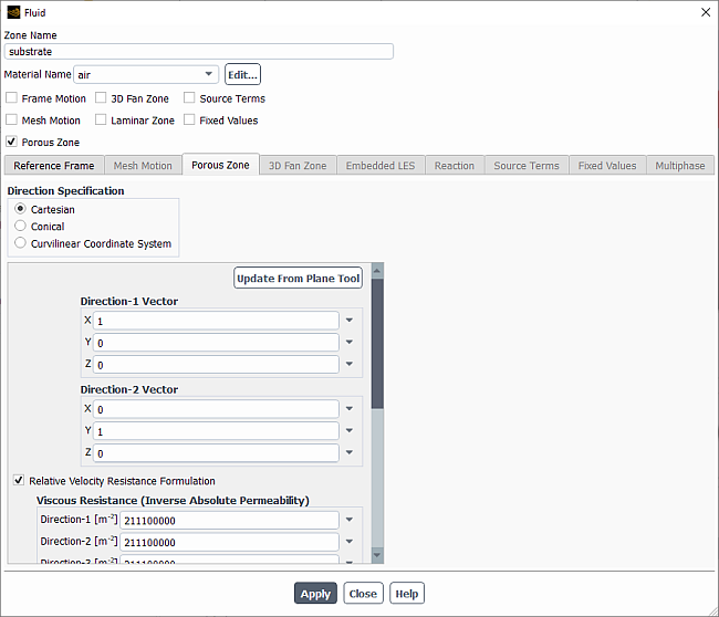
As mentioned in Overview, a porous zone is modeled as a special type of fluid zone. To indicate that the fluid zone is a porous region, enable the Porous Zone option in the Fluid dialog box. The dialog box will expand to show the porous media inputs (as shown in Figure 7.22: The Fluid Dialog Box for a Porous Zone).
In a coupled analysis involving Fluent and System Coupling, a porous jump boundary of zero-thickness next to the porous zone can be used to transfer data between the porous zone and the System Coupling system. For more about System Coupling and the variable transferred from a porous jump boundary, see Performing System Coupling Simulations Using Fluent.
The Cell Zone Conditions task page contains a Porous Formulation region where you can instruct Ansys Fluent to use either a superficial or physical velocity in the porous medium simulation. By default, the velocity is set to Superficial Velocity. For details about using the Physical Velocity formulation, see Modeling Porous Media Based on Physical Velocity.
To define the fluid that passes through the porous medium, select the appropriate fluid in the Material Name drop-down list in the Fluid Dialog Box. If you want to check or modify the properties of the selected material, you can click to open the Edit Material dialog box; this dialog box contains just the properties of the selected material, not the full contents of the standard Create/Edit Materials dialog box.
Important: If you are modeling species transport or multiphase flow, the Material Name list will not appear in the Fluid dialog box. For species calculations, the mixture material for all fluid/porous zones will be the material you specified in the Species Model Dialog Box. For multiphase flows, the materials are specified when you define the phases, as described in Defining the Phases for the VOF Model.
If you are modeling species transport with reactions, you can enable reactions in a porous zone by turning on the Reaction option in the Fluid dialog box and selecting a mechanism in the Reaction Mechanism drop-down list.
If your mechanism contains wall surface reactions, you also must specify a value for the Surface-to-Volume
Ratio. This value is the surface area of the pore walls per unit volume ( ), and can be thought of as a measure of catalyst loading. With this value, Ansys Fluent can calculate the total
surface area on which the reaction takes place in each cell by multiplying
), and can be thought of as a measure of catalyst loading. With this value, Ansys Fluent can calculate the total
surface area on which the reaction takes place in each cell by multiplying  by the volume of the cell and the porosity. See Defining Zone-Based Reaction Mechanisms for details about
defining reaction mechanisms. See Wall Surface Reactions and Chemical Vapor Deposition for details about wall surface reactions.
by the volume of the cell and the porosity. See Defining Zone-Based Reaction Mechanisms for details about
defining reaction mechanisms. See Wall Surface Reactions and Chemical Vapor Deposition for details about wall surface reactions.
Note: The wall surface reactions in porous medium are allowed only for the pressure-based solver.
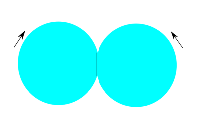
For cases involving moving meshes, dynamic meshes or moving reference frames (MRF), the Relative Velocity Resistance Formulation option allows you to better predict porous media sources. The porous media source terms are calculated using relative velocities in the porous zone. For more information, see Momentum Equations for Porous Media. The Relative Velocity Resistance Formulation option works well for cases with moving and stationary porous media. It is turned on by default.
Note the following limitation when using the Relative Velocity Resistance Formulation option:
The relative velocity resistance formulation is not supported with axisymmetric-swirl when there are non-zero swirl resistances.
Note: In Ansys Fluent 6.3, this option was only supported for moving mesh and MRF (with the exception of power law for modeling porous sources). Currently, this option also supports dynamic mesh and takes care of proper treatment of porous sources using power law.
The viscous and inertial resistance coefficients are both defined in the same manner. The basic approach for defining the coefficients using a Cartesian coordinate system is to define one direction vector (Direction-1 Vector) in 2D or two direction vectors (Direction-1 Vector and Direction-2 Vector) in 3D, and then specify the viscous and/or inertial resistance coefficients in each direction. The Direction-1 Vector usually represents the primary flow direction (parallel to the porous zone axis), and the other two directions represent the transverse directions.
Ansys Fluent automatically determines the second direction vector in 2D or the third direction vector in 3D, which is not explicitly defined:
In 2D, the second direction is normal to the plane defined by the Direction-1 Vector and the z-direction vector.
In 3D, the third direction is normal to the plane defined by the Direction-1 Vector and Direction-2 Vector. Note that the Direction-2 Vector must be normal to the Direction-1 Vector. If you fail to specify two normal directions, the Ansys Fluent solver will orthogonalize the direction specification by removing the projection of the Direction-2 Vector on the Direction-1 Vector before computing the third mutually orthogonal direction. You should therefore be certain that the first direction is correctly specified.
If the porous zone faces are not aligned with the global Cartesian axis, you can use the plane tool in 3D or the line tool in 2D for the direction vector definitions as further described.
You can also define the viscous and/or inertial resistance coefficients in each direction using a user-defined function
(UDF). The user-defined options become available in the corresponding drop-down list when the UDF has been created and loaded
into Ansys Fluent. Note that the coefficients defined in the UDF must utilize the DEFINE_PROFILE macro.
For more information on creating and using user-defined function, see the Fluent Customization Manual.
If you are modeling axisymmetric swirling flows, you can specify an additional direction component for the viscous and/or inertial resistance coefficients. This direction component is always tangential to the other two specified directions. This option is available for both density-based and pressure-based solvers.
In 3D, it is also possible to define the coefficients using a conical (or cylindrical) coordinate system, as described below.
Important: Note that the viscous and inertial resistance coefficients are generally based on the superficial velocity of the fluid in the porous media.
The procedure for defining resistance coefficients is as follows:
Define the direction vectors.
To use a Cartesian coordinate system, simply specify the Direction-1 Vector and, for 3D, the Direction-2 Vector. The unspecified direction will be determined as described above. These direction vectors correspond to the principle axes of the porous media.
Note: The units for the inertial resistance coefficients (Direction-1 Vector and Direction-2 Vector) is the inverse of length. Should you want to define different units, you can do so by opening the Units dialog box and selecting resistance from the Quantities list.
For some problems in which the principal axes of the porous medium are not aligned with the coordinate axes of the domain, you may not know a priori the direction vectors of the porous medium. In such cases, the plane tool (available via the Plane Surface dialog box) in 3D or the line tool (available via the Line/Rake Surface dialog box) in 2D can help you to determine these direction vectors.
Open the Plane Surface dialog box in 3D or the Line/Rake Surface dialog box in 2D to enable the plane or line tool.
Rotate the axes of the tool appropriately until they are aligned with the porous medium. You may want to move the plane tool (or the line tool) onto the boundary of the porous region. (Follow the instructions in Using the Plane Tool or Using the Line Tool for initializing the tool to a position on an existing surface.)
Once the axes are aligned, click the or button in the Fluid dialog box. Ansys Fluent will automatically set the Direction-1 Vector to the direction of the red arrow of the tool, and (in 3D) the Direction-2 Vector to the direction of the green arrow.
Important: The Plane Surface Dialog Box or the Line/Rake Surface Dialog Box must be open for the plane or line tool to be active.
To use a conical coordinate system (for example, for an annular, conical filter element), follow the steps below. This option is available only in 3D cases.
Turn on the Conical option.
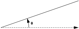
Set the Cone Half Angle (the angle between the cone’s axis and its surface, shown in Figure 7.23: Cone Half Angle). To use a cylindrical coordinate system, set the Cone Half Angle to 0.
Specify the Cone Axis Vector and Point on Cone Axis. The cone axis is specified as being in the direction of the Cone Axis Vector (unit vector), and passing through the Point on Cone Axis. The cone axis may or may not pass through the origin of the coordinate system.
For some problems in which the axis of the conical filter element is not aligned with the coordinate axes of the domain, you may not know a priori the direction vector of the cone axis and coordinates of a point on the cone axis. In such cases, the plane tool can help you to determine the cone axis vector and point coordinates. One method is as follows:
Select a boundary zone of the conical filter element that is normal to the cone axis vector in the drop-down list next to the button.
Click the button. Ansys Fluent will automatically “snap” the plane tool onto the boundary. It will also set the Cone Axis Vector and the Point on Cone Axis. (Note that you will still have to set the Cone Half Angle yourself.)
An alternate method is as follows:
Move the plane tool onto the boundary of the porous region. (Follow the instructions in Using the Plane Tool for moving the tool to a position on an existing surface.) Open the Plane Surface dialog box to enable the plane tool.
Rotate and translate the axes of the tool appropriately until the red arrow of the tool is pointing in the direction of the cone axis vector and the origin of the tool is on the cone axis.
Once the axes and origin of the tool are aligned, click the button in the Fluid dialog box. Ansys Fluent will automatically set the Cone Axis Vector and the Point on Cone Axis. (Note that you will still have to set the Cone Half Angle yourself.)
Open the Plane Surface Dialog Box or the Line/Rake Surface Dialog Box to make the plane or line tool appear.
To use a curvilinear coordinate system (such as for a winding or coil), follow the steps below. This option is available only in 3D cases.
Under Direction Specification, select Curvilinear Coordinate System.
For Coordinate System, select an already created curvilinear coordinate system or you can create a new one by clicking New.... For details on creating a curvilinear coordinate system, see Curvilinear Coordinate Systems.
For Viscous Resistance and Inertial Resistance, the direction components will correspond to the directions defined for the chosen curvilinear coordinate system.
Under Viscous Resistance, specify the viscous resistance coefficient
 in each direction.
Under Inertial Resistance, specify the inertial resistance coefficient
 in each direction. (You can scroll down with the scroll bar to view these inputs.)
For porous media cases containing highly anisotropic inertial resistances, enable Alternative Formulation under Inertial Resistance. The Alternative Formulation option provides better stability to the calculation when your porous medium is anisotropic. The pressure loss through the medium depends on the magnitude of the velocity vector of the i th component in the medium. Using the formulation of Equation 7–6 yields the expression below:

(7–24)
Whether or not you use the Alternative Formulation option depends on how well you can fit your experimentally determined pressure drop data to the Ansys Fluent model. For example, if the flow through the medium is aligned with the mesh in your Ansys Fluent model, then it will not make a difference whether or not you use the formulation. In general, however, the default and the Alternative Formulation are not equivalent, and solution differences can occur when switching between the two options.
Note: After you change the status of the Alternative Formulation option, you need to rerun the simulation to obtain consistent force reports and cumulative plots (Cumulative Force, Moment, and Coefficients Plots) for lift, drag, moments, and corresponding coefficients computed on porous zones. This is because the porous force contribution is always obtained on demand by recomputing the porous sources used in the momentum equations, which can change with enabling or disabling the Alternative Formulation option.
For more information about simulations involving highly anisotropic porous media, see Solution Strategies for Porous Media.
Important: Note that the alternative formulation is compatible only with the pressure-based solver.
If you are using the Conical specification method, Direction-1 is the tangential direction of the cone, Direction-2 is the normal to the cone surface (radial (
 ) direction for a cylinder), and Direction-3 is the circumferential
(
) direction for a cylinder), and Direction-3 is the circumferential
( ) direction.
In 3D there are three possible categories of coefficients, and in 2D there are two:
In the isotropic case, the resistance coefficients in all directions are the same (for example, a sponge). For an isotropic case, you must explicitly set the resistance coefficients in each direction to the same value.
When (in 3D) the coefficients in two directions are the same and those in the third direction are different or (in 2D) the coefficients in the two directions are different, you must be careful to specify the coefficients properly for each direction. For example, if you had a porous region consisting of cylindrical straws with small holes in them positioned parallel to the flow direction, the flow would pass easily through the straws, but the flow in the other two directions (through the small holes) would be very little. If you had a plane of flat plates perpendicular to the flow direction, the flow would not pass through them at all; it would instead move in the other two directions.
In 3D the third possible case is one in which all three coefficients are different. For example, if the porous region consisted of a plane of irregularly-spaced objects (for example, pins), the movement of flow between the blockages would be different in each direction. You would therefore need to specify different coefficients in each direction.
Methods for deriving viscous and inertial loss coefficients are described in the sections that follow.
When you use the porous media model, you must remember that the porous cells in Ansys Fluent are 100% open,
and that the values that you specify for  and/or
  must be based on this assumption. Suppose, however, that you know how the pressure drop varies with the
velocity through the actual device, which is only partially open to flow. The following exercise is designed to show you how
to compute a value for
must be based on this assumption. Suppose, however, that you know how the pressure drop varies with the
velocity through the actual device, which is only partially open to flow. The following exercise is designed to show you how
to compute a value for  which is appropriate for the Ansys Fluent model.
Consider a perforated plate that has 25% area open to flow. The pressure drop through the plate is known to be 0.5 times the
dynamic head in the plate. The loss factor,  , defined as
 | (7–25) |
is therefore 0.5, based on the actual fluid velocity in the plate, that is, the velocity through the 25% open area. To
compute an appropriate value for  , note that in the Ansys Fluent model:
The velocity through the perforated plate assumes that the plate is 100% open.
The loss coefficient must be converted into dynamic head loss per unit length of the porous region.
Noting item 1, the first step is to compute an adjusted loss factor,  , which would be based on the velocity of a 100% open area:
 | (7–26) |
or, noting that for the same flow rate,  ,
,
 | (7–27) |
The adjusted loss factor has a value of 8. Noting item 2, you must now convert this into a loss coefficient per unit
thickness of the perforated plate. Assume that the plate has a thickness of 1.0 mm ( m). The inertial loss factor would then be
 | (7–28) |
Note that, for anisotropic media, this information must be computed for each of the 2 (or 3) coordinate directions.
As a second example, consider the modeling of a packed bed. In turbulent flows, packed beds are modeled using both a permeability and an inertial loss coefficient. One technique for deriving the appropriate constants involves the use of the Ergun equation [42], a semi-empirical correlation applicable over a wide range of Reynolds numbers and for many types of packing:
 | (7–29) |
When modeling laminar flow through a packed bed, the second term in the above equation may be dropped, resulting in the Blake-Kozeny equation [42]:
 | (7–30) |
In these equations,  is the viscosity,
  is the mean particle diameter,
  is the bed depth, and
  is the void fraction, defined as the volume of voids divided by the volume of the packed bed region.
Comparing Equation 7–4 and Equation 7–6 with Equation 7–29, the permeability and inertial loss coefficient in each component direction may be identified as
is the void fraction, defined as the volume of voids divided by the volume of the packed bed region.
Comparing Equation 7–4 and Equation 7–6 with Equation 7–29, the permeability and inertial loss coefficient in each component direction may be identified as
 | (7–31) |
and
 | (7–32) |
As a third example we will take the equation of Van Winkle et al. [118] [150] and show how porous media inputs can be calculated for pressure loss through a perforated plate with square-edged holes.
The expression, which is claimed by the authors to apply for turbulent flow through square-edged holes on an equilateral triangular spacing, is
 | (7–33) |
| where | |
 = mass flow rate through the plate = mass flow rate through the plate | |
 = the free area or total area of the holes = the free area or total area of the holes | |
 = the area of the plate (solid and holes) = the area of the plate (solid and holes) | |
 = a coefficient that has been tabulated for various Reynolds-number ranges and for various = a coefficient that has been tabulated for various Reynolds-number ranges and for various
 | |
 = the ratio of hole diameter to plate thickness = the ratio of hole diameter to plate thickness |
for  and for
  the coefficient
  takes a value of approximately 0.98, where the Reynolds number is based on hole diameter and velocity in the
holes.
takes a value of approximately 0.98, where the Reynolds number is based on hole diameter and velocity in the
holes.
Rearranging Equation 7–33, making use of the relationship
 | (7–34) |
and dividing by the plate thickness,  , we obtain
 | (7–35) |
where  is the superficial velocity (not the velocity in the holes). Comparing with Equation 7–6 is seen that, for the direction normal to the plate, the constant
  can be calculated from
 | (7–36) |
Consider the problem of laminar flow through a mat or filter pad which is made up of randomly-oriented fibers of glass wool. As an alternative to the Blake-Kozeny equation (Equation 7–30) we might choose to employ tabulated experimental data. Such data is available for many types of fiber [71].
| Volume Fraction of Solid Material | Dimensionless Permeability  of Glass Wool of Glass Wool
|
|---|---|
| 0.262 | 0.25 |
| 0.258 | 0.26 |
| 0.221 | 0.40 |
| 0.218 | 0.41 |
| 0.172 | 0.80 |
where  and
and  is the fiber diameter.
  , for use in Equation 7–4, is easily computed for a given fiber diameter and volume
fraction.
, for use in Equation 7–4, is easily computed for a given fiber diameter and volume
fraction.
Experimental data that is available in the form of pressure drop against velocity through the porous component, can be
extrapolated to determine the coefficients for the porous media. To effect a pressure drop across a porous medium of
thickness,  , the coefficients of the porous media are determined in the manner described below.
If the experimental data is:
| Velocity (m/s) | Pressure Drop (Pa) |
|---|---|
| 20.0 | 197.8 |
| 50.0 | 948.1 |
| 80.0 | 2102.5 |
| 110.0 | 3832.9 |
then an  curve can be plotted to create a trendline through these points yielding the following equation
 | (7–37) |
where  is the pressure drop and
  is the velocity.
Important: Although the best fit curve may yield negative coefficients, it should be avoided when using the porous media model in Ansys Fluent.
Note that a simplified version of the momentum equation, relating the pressure drop to the source term, can be expressed as
 | (7–38) |
or
 | (7–39) |
Hence, comparing Equation 7–37 to Equation 7–2, yields the following curve coefficients:
 | (7–40) |
with  kg/
kg/  , and a porous media thickness,
  , assumed to be 1 m in this example, the inertial resistance factor,
  .
.
Likewise,
 | (7–41) |
with  , the viscous inertial resistance factor,
  .
.
Important: Note that this same technique can be applied to the porous jump boundary condition. Similar to the case of the porous
media, you have to take into account the thickness of the medium  . Your experimental data can be plotted in an
  curve, yielding an equation that is equivalent to Equation 7–152. From there,
you can determine the permeability
curve, yielding an equation that is equivalent to Equation 7–152. From there,
you can determine the permeability  and the pressure jump coefficient
  .
.
If you choose to use the power-law approximation of the porous-media momentum source term (Equation 7–3), the only inputs required are the coefficients  and
and  . Under Power Law Model in the Fluid dialog box, enter the values
for C0 and C1. Note that the power-law model can be used in conjunction with the
Darcy and inertia models.
. Under Power Law Model in the Fluid dialog box, enter the values
for C0 and C1. Note that the power-law model can be used in conjunction with the
Darcy and inertia models.
C0 must be in SI units, consistent with the value of C1.
To define the porosity, scroll down below the resistance inputs in the Fluid dialog box, and set the
Porosity under Fluid Porosity. Note that the value of the
Porosity must be in the range of 0 – 1 ;
furthermore, the lower and upper limits (that is, 0 and 1, respectively) are
not allowed for the non-equilibrium thermal model.
You can also define the porosity using a user-defined function (UDF). The user-defined option becomes available in the
corresponding drop-down list when the UDF has been created and loaded into Ansys Fluent. Note that the porosity defined in the UDF
must utilize the DEFINE_PROFILE macro. For more information on creating and using user-defined
functions, see the separate Fluent Customization Manual.
The porosity,  , is the volume fraction of fluid within the porous region (that is, the open volume fraction of the medium).
The porosity is used in the prediction of heat transfer in the medium, as described in Treatment of the Energy Equation in Porous Media, and in the time-derivative term in the scalar transport equations for unsteady flow, as described in Effect of Porosity on Transient Scalar Equations. It also impacts the calculation of reaction source terms and body forces in the
medium. These sources will be proportional to the fluid volume in the medium. If you want to represent the medium as
completely open (no effect of the solid medium), you should set the porosity equal to 1.0 (the default). When the porosity is
equal to 1.0, the solid portion of the medium will have no impact on heat transfer or thermal/reaction source terms in the
medium.
, is the volume fraction of fluid within the porous region (that is, the open volume fraction of the medium).
The porosity is used in the prediction of heat transfer in the medium, as described in Treatment of the Energy Equation in Porous Media, and in the time-derivative term in the scalar transport equations for unsteady flow, as described in Effect of Porosity on Transient Scalar Equations. It also impacts the calculation of reaction source terms and body forces in the
medium. These sources will be proportional to the fluid volume in the medium. If you want to represent the medium as
completely open (no effect of the solid medium), you should set the porosity equal to 1.0 (the default). When the porosity is
equal to 1.0, the solid portion of the medium will have no impact on heat transfer or thermal/reaction source terms in the
medium.
You can model heat transfer in the porous material, with or without the assumption of thermal equilibrium between the medium and the fluid flow. Note that heat transfer is not available for inviscid flow.
To specify that the porous medium and the fluid flow are in thermal equilibrium, scroll down below the resistance inputs in the Fluid dialog box to the Heat Transfer Settings group box and select Equilibrium from the Thermal Model list (this is the default selection). Then you must specify the material contained in the porous medium by selecting the appropriate solid in the Solid Material Name drop-down list.
If you want to check or modify the properties of the selected material, you can click to
open the Edit Material dialog box; this dialog box contains just the properties of the selected
material, not the full contents of the standard Create/Edit Materials dialog box. You can define the
Thermal Conductivity of the porous material using a user-defined function (UDF), in order to define a
non-isotropic thermal conductivity. The user-defined option becomes available in the corresponding drop-down list when the
UDF has been created and loaded into Ansys Fluent. Note that the non-isotropic thermal conductivity defined in the UDF must
utilize the DEFINE_PROPERTY macro. For more information on creating and using user-defined
function, see the separate Fluent Customization Manual.
Note: The non-equilibrium thermal model is incompatible with the density-based solver.
The assumption of thermal equilibrium between the solid medium and the fluid flow is not appropriate for all simulations, as the presence of different geometric length scales (for example, pore sizes) and physical properties of solid and liquid phases may result in local temperature differences between the phases. Examples of when a non-equilibrium thermal model may be suitable include the simulation of light-off for exhaust after-treatment, fuel cells, catalytic converters, and so on.
The non-equilibrium thermal model available for porous media in Ansys Fluent is based on a dual cell approach. This approach
is referred to as “dual cell” because it involves a second solid cell zone that overlaps (that is, is
spatially coincident with) the porous fluid zone; the two zones are solved simultaneously and are coupled only through
heat transfer. Ansys Fluent can automatically create a solid zone for you that is a duplicate of the porous fluid zone;
otherwise, you can create a duplicate cell zone manually using the
mesh/modify-zones/copy-move-cell-zone text command before you enable the non-equilibrium thermal
model, or make sure that the mesh you read contains two cell zones in the region where the porous medium will be defined.
You should ensure that the duplicate zone is defined as a solid zone, and that the two zones have similar levels of mesh
refinement (as one-to-one mapping will be employed between the cell centroids of the fluid zone and the solid
zone).
Important: When setting up both the porous fluid zone and the overlapping solid zone, note that the non-equilibrium thermal model is not supported for zones that undergo (or are adjacent to zones that undergo) changes to the geometry or mesh, such as dynamic mesh zones or zones that undergo hanging node adaption, utilize the mesh morpher/optimizer, or are involved in fluid-structure interaction (FSI) applications.
The instructions that follow assume you have already performed steps 1–7 in User Inputs for Porous Media. Before you enable the non-equilibrium thermal model, click in the Fluid dialog box, in order to save your settings in the Porous Zone tab; note that if you do not save your settings, they will be reset to the default values when you enable the non-equilibrium thermal model. Then reopen the Fluid dialog box and scroll down below the resistance inputs in the Porous Zone tab. Select Non-Equilibrium from the Thermal Model list in the Heat Transfer Settings group box (see Figure 7.24: The Heat Transfer Settings Group Box of the Fluid Dialog Box); this will enable the dual cell approach and display the associated GUI input controls. If a solid zone that is spatially coincident with the porous fluid zone does not already exist, use the Question dialog box that opens to automatically create one. The name of the newly created solid cell zone will then be displayed in the Solid Zone text box of the Fluid dialog box.
Important: Note that the Non-Equilibrium option button is not available if a radiation and/or multiphase model is enabled, as such a combination is not supported.
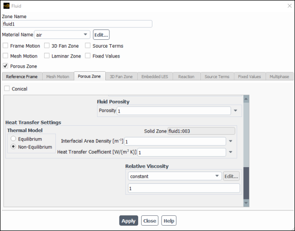
Next, define  and
and  (as described in Non-Equilibrium Thermal Model Equations) for Interfacial Area Density
and Heat Transfer Coefficient, respectively; you can define these settings as a
Constant, a New Input Parameter..., or as a user-defined function. The
user-defined option becomes available in the corresponding drop-down list when the UDF has been
created and loaded into Ansys Fluent. Note that the UDF must utilize the
(as described in Non-Equilibrium Thermal Model Equations) for Interfacial Area Density
and Heat Transfer Coefficient, respectively; you can define these settings as a
Constant, a New Input Parameter..., or as a user-defined function. The
user-defined option becomes available in the corresponding drop-down list when the UDF has been
created and loaded into Ansys Fluent. Note that the UDF must utilize the DEFINE_PROFILE macro. For
more information on creating and using user-defined functions, see the separate Fluent Customization Manual.
When you are finished setting up the porous fluid zone, you should verify that the solid zone created in the previous
step has the appropriate settings. Note the name of the zone displayed in the Solid Zone text box of
the Heat Transfer Settings group box (see Figure 7.24: The Heat Transfer Settings Group Box of the Fluid Dialog Box), and then
double-click that zone in the Zone list of the Cell Zone Conditions task page to
open the Solid dialog box. Then, verify that an appropriate selection is made for Material
Name. If you want to check or modify the properties of the selected material, you can click
to open the Edit Material dialog box; this dialog box contains just
the properties of the selected material, not the full contents of the standard Create/Edit Materials
dialog box. You can define the Thermal Conductivity of the solid material using a user-defined
function (UDF), in order to define a non-isotropic thermal conductivity. The user-defined option becomes available in the
corresponding drop-down list when the UDF has been created and loaded into Ansys Fluent. Note that the non-isotropic thermal
conductivity defined in the UDF must utilize the DEFINE_PROPERTY macro. For more information on
creating and using user-defined functions, see the separate Fluent Customization Manual.
Important: For transient simulations using the Non-Equilibrium Thermal Model with low porosity (typically < 0.2), it is recommended to increase the Solid Time Step Size as described in Specifying the Solid Time Step Size. A value ~1s or the Automatic option can help with solution stability and convergence.
Note that when postprocessing simulations that utilize the non-equilibrium thermal model, you can display the energy source due to the temperature difference between the fluid and solid zones using the Non-Equilibrium Thermal Model Source variable in the Temperature... category. Furthermore, attention must be paid to the fact that there are overlapping cell zones (that is, a fluid and a solid zone) in the porous region. For example:
When creating an isosurface and making selections from the From Zones selection list of the Iso-Surface dialog box, you should never select both the porous fluid zone and the overlapping solid zone at the same time. Note that if no selections are made in this list, then all the cell zones are selected.
When making selections from the Surfaces list of the Contours dialog box, you should not select a surface that is associated with the porous fluid zone and a surface associated with the overlapping solid zone at the same time, if those surfaces are spatially coincident.
When postprocessing the thermal conductivity property in the porous region, the value that is reported for the fluid zone is the thermal conductivity of the fluid material scaled by the porosity (
 ) and for the overlapping solid zone the value reported is the thermal conductivity of the solid
zone scaled by the complement of the porosity (
) and for the overlapping solid zone the value reported is the thermal conductivity of the solid
zone scaled by the complement of the porosity ( ); where
  is the porosity,
  is the fluid phase thermal conductivity (including the turbulent contribution,
  ), and
  is the solid medium thermal conductivity.
The relative viscosity can be used to account for the effect of the porous media on the diffusion term in the momentum
equation. By default, the relative viscosity is set to a constant value of 1 (that is, the effective viscosity is equal to the
molecular viscosity). You can choose to model the relative viscosity using one of the models described in Relative Viscosity in Porous Media, or you can specify a user-defined function using a
DEFINE_PROPERTY macro.
When you define multiple porous zones, the last value you enter for the relative viscosity will be applied to compute the
effective viscosity for all porous zones in your simulation. If you want to simulate different effective viscosities in
different porous zones, specify the Viscosity property of the porous material directly via user-defined
function using the DEFINE_PROPERTY macro (in the Create/Edit Materials dialog
box).
The relative permeability of a phase denotes its ability to transmit the phase material when its saturation (volume fraction) is less than 100%.
Reservoir engineers often resort to empirical models or measurement curves to determine the relative and, therefore, the effective permeabilities. In Fluent, the Corey power law model [27] is available to account for the relative permeability for the two-phase flow through porous media. The Corey correlations of the relative permeability can be represented as follows:
 | (7–42) |
| where: | |
 is the reference phase relative permeability is the reference phase relative permeability | |
 is the normalized saturation in the q th phase is the normalized saturation in the q th phase | |
 is the Corey exponent for the q th phase is the Corey exponent for the q th phase |
In Fluent the phase saturation is the phase volume fraction. Thus  can be expressed as:
 | (7–43) |
where  and
and  are the volume fraction and the volume fraction residual in
the q th phase, respectively.
are the volume fraction and the volume fraction residual in
the q th phase, respectively.
For the two-phase oil-water flow in a water-wet-system, the relative permeabilities can be obtained from:
 | (7–44) |
where:
Subscripts  and and  refer to the water and oil phases, respectively refer to the water and oil phases, respectively |
 and and  are the reference phase relative permeabilities for the
wetting and non-wetting phases, respectively are the reference phase relative permeabilities for the
wetting and non-wetting phases, respectively |
 and and  are the Corey exponents for the two phases are the Corey exponents for the two phases |
The Corey correlation is often used for approximation of the relative permeabilities, particularly for water flooding type scenarios. The relative permeability curves of the oil (or the non-wetting phase) is usually an S-shaped curve and of the water (or the wetting phase) is a concave upward curve.
Alternatively, if relative permeability data for one or two phases are available as tabular functions of other solution variables, you can use generic text files to input such data to define phase relative permeability as described in Reading Files in Tabular Format.
To model the relative permeability in Ansys Fluent:
Set parameters for the mixture phase.
Note: The phase can be selected from the Phase drop-down list either in the Cell Zone Conditions task page or in the Fluid dialog box.
In the Fluid dialog box, make sure that mixture is selected from the Phase drop-down list.
In the Porous Zone tab, under Relative Permeability, select Corey Model.
From the drop-down lists, select Wetting Phase and Non Wetting Phase.
Important: Although Equation 7–42 through Equation 7–44 are valid for any given phase, care must be exercised in defining the wetting and non-wetting phases.
Click Apply.
Set conditions for the wetting phase.
In the Fluid dialog box, make sure that the wetting phase is selected from the Phase drop-down list.
In the Porous Zone tab, specify the following parameters in the Wetting Phase Relative Permeability group box:
- Minimum Relative Permeability
sets a lower limit for the relative permeability for the wetting phase. A low value increases impact of the resistance due to relative permeability effects on the flow. This helps to avoid saturation overshoots and undershoots (that is, phase saturation dropping below residual values) in simulations carried out for a long period of time. The default value is 1.e-8. The default should work for most cases, but may be lowered in case undershoot problems persist.
- Reference Relative Permeability
is
in Equation 7–44. This parameter is
available only when the tabular
option is disabled.- Corey Exponent
is
in Equation 7–44.- Residual Saturation
is the residual volume fraction of the wetting phase. This parameter is available only when the tabular option is disabled.
If, instead, you wish to specify the relative permeability parameters for the wetting phase in the tabular format, follow these steps:
Select tabular and click .
Note: Prior to using the tabular option, you must read a text file containing phase relative permeability data as described in Capillary Pressure Data in a Tabular Format.
In the Table Input dialog box that opens, select the table appropriate for your fluid zone from the Table List and the names of the columns from the Saturation (VOF) and Relative Permeability selection lists.
See Capillary Pressure Data in a Tabular Format for details about the text file format.
Click Apply.
Similarly, set conditions for the non-wetting phase.
In the Fluid dialog box, make sure that the non-wetting phase is selected from the Phase drop-down list.
In the Porous Zone tab, specify the following parameters in the Non Wetting Phase Relative Permeability group:
- Minimum Relative Permeability
sets a lower limit for the relative permeability for the non-wetting phase. This item is similar to Minimum Relative Permeability for the wetting phase.
- Reference Relative Permeability
is
in Equation 7–44. This parameter is
available only when the tabular
option is disabled.- Corey Exponent
is
in Equation 7–44.- Residual Saturation
is the residual volume fraction of the non-wetting phase. This parameter is available only when the tabular option is disabled.
If, instead, you wish to specify the relative permeability parameters for the non-wetting phase in the tabular format, select tabular. The inputs are similar to the tabular specification for the wetting phase.
Click Apply.
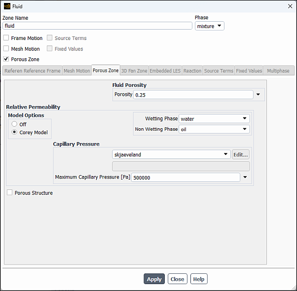
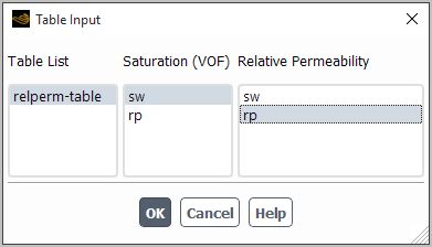
On rare occasions, the saturation may still fall below residual saturation. You can fix the affected phase to its residual saturation and allow the other phase to pass through normally by issuing the following text commands:
solve/set/multiphase-numerics/porous-media/relative-permeability
enable fix option below residual saturation? [no] yes
Note: The previous text command is not supported for cases that use the tabular specification method for phase relative permeability.
When using the Eulerian multiphase model, you can optionally specify a sub-model for capillary pressure.
When two or more phases are present in pores, one of the phase (usually water) has a preference for the pore surfaces. This phase is referred to as the wetting phase, while the other phase is called the non-wetting phase. The boundary between the phases present in a porous medium is also curved, due to interfacial tension between the fluid, and this gives rise to a difference in the pressure across the interface:
 | (7–45) |
where  and
and  are the non-wetting and wetting phase pressures, respectively. The difference,
  is the capillary pressure. It presents a significant driving force under the conditions of low flow pressure
and high volume fraction.
is the capillary pressure. It presents a significant driving force under the conditions of low flow pressure
and high volume fraction.
At the pore scale, capillary pressure depends primarily on the pore geometric characteristics (sizes, distributions, etc.), interfacial tensions and wettability (contact angles). At the Macro scale the capillary pressure is generally assumed to be a function of the saturation of the wetting fluid:
 | (7–46) |
Its value is often obtained either by measurements or correlations.
In Fluent, the capillary pressure effect is modeled as an additional source term in the wetting phase. Additional information is provided in the following sections:
The Brooks-Corey model [27] proposed the following relationship for capillary pressure for primary drainage, in which the porous media initially saturated with water is invaded with oil phase:
 | (7–47) |
where  is the resulting normalized (effective) saturation:
 | (7–48) |
where  and
and  are the minimum and maximum volume fraction (saturation) values, respectively. By default
 and
and  where
where  is the residual saturation of phase
  The value of
  is limited to values greater than 0.001 in order to avoid an infinite value for capillary
pressure.
is limited to values greater than 0.001 in order to avoid an infinite value for capillary
pressure.
In order to solve Equation 7–47, the entry pressure,  , and the parameter
  related to the pore size are required. The default values in Fluent are
  and
and  which are appropriate for air-water flow in sand [29].
Another well established parametric model was proposed by van Genuchten [48]:
 | (7–49) |
where  is the entry pressure.
  is the pore size distribution and
  . The default values inFluent are
  and
and  which are appropriate for air-water flow in sand [29].
The J-function was developed by Leverett in an attempt to extend the pore-scale capillary pressure formulation by Washburn [29] to a Macro-scale capillary pressure model. Leverett proposed that the averaged pore radius can be expressed in terms of porosity and permeability:
 | (7–50) |
Furthermore, he acknowledged that the capillary pressure should depend on porosity and permeability. By analogy to the Washburn equation, he developed a dimensionless J-function [85]:
 | (7–51) |
 | (7–52) |
where  is the surface tension,
  is the wetting or contact angle, and
  and
and  are fitting parameters. Various empirical J-functions can be developed to estimate capillary pressure.
In the Fluent, the following formulation is used:
are fitting parameters. Various empirical J-functions can be developed to estimate capillary pressure.
In the Fluent, the following formulation is used:
 | (7–53) |
This is the same formulation as is used in the Fluent Fuel Cell Module (see Liquid Water Formation, Transport, and its Effects (Low-Temperature PEMFC Only) in the Fluent Theory Guide).
All of the above-mentioned capillary pressure models (Brooks-Corey, Van-Genuchten, Leverett J-Function) are limited to primary drainage processes. Water saturation decreases in a primary drainage process. To model a displacement process where flooding is important, such as water-drive, models that describe imbibition are required. However, most reservoirs are mixed wettabilty and for these systems a more comprehensive model that describes both drainage and imbibition processes is required. The Skjaeveland model for capillary pressure encompasses these features.
The Skjaeveland model [145] for capillary pressure treats the two fluids symmetrically for wettability. The Skjaeveland capillary pressure curve is defined by Equation 7–54.
 | (7–54) |
Where  is the capillary pressure of the
  phase,
  and
and  are fitting parameters,
  and
and  are constants, and
  and
and  are the volume fractions of the two phases.
  and
and  subscripts refer to wetting and non-wetting phases, respectively.
The positive part of the capillary pressure curve is defined by
 and
and  .
.  and
and  define the negative portion of the capillary pressure
curve. The effects of varying
define the negative portion of the capillary pressure
curve. The effects of varying  ,
,  ,
,  , and
, and  on the capillary pressure curve are shown in Figure 7.27: Skjaeveland Correlation Behavior
[145].
on the capillary pressure curve are shown in Figure 7.27: Skjaeveland Correlation Behavior
[145].
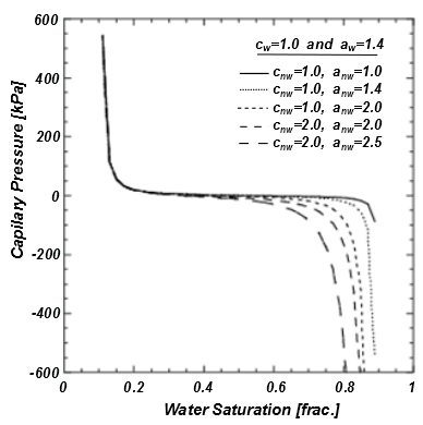
Figure 7.27: Skjaeveland Correlation Behavior shows that there is a lot of flexibility in the capillary
pressure curve. You can add further flexibility to the capillary pressure curve by estimating the residual oil saturation.
Note that by varying  and
and  you can modify the cross-over point (while keeping
  and
and  unchanged).
|
Parameter |
Default Value |
|---|---|
|
|
9.e5 |
|
|
9.e5 |
|
|
0.05 |
|
|
0.05 |


Often, field data for capillary pressure are available as tabular functions of other solution variables. In, Ansys Fluent, you can use a tabular method to specify capillary pressure. Multiple files can be used to specify zone-specific properties, for example, different models for capillary pressure for different zones.
The text file format and the table reading procedure are described in Reading Files in Tabular Format.
An example of the data file for the capillary pressure variable is shown below.
Default-Skjaevland-Model
Sw          Pc
0.2122      195399.0883
0.2245      156423.6016
0.2367      134012.8962
0.249       117936.4991
0.2612      105469.0929
0.2735      95079.83957
0.2857      86245.04955
0.298       78405.02466
Row 1 – The name of the table. The name should not exceed 128 characters and contain no spaces. For example, Default-Skjaevland-Model and Default_Skjaevland_Model are acceptable names.
Row 2 – Column names for the table input data (Sw and Pc in the above example).
Row 3 and all consecutive rows – Data points of the saturation and the corresponding capillary pressure values as a function of the saturation.
See Capillary Pressure Usage for more information on tabular input for capillary pressure.
To model the capillary pressure:
In the Fluid dialog box for the phase mixture, in the Porous Zone tab, select Corey Model (Model Options group box).
Select a model from the drop-down list under Capillary Pressure. You can choose from the following models:
brooks-corey
van-genuchten
leverett-j-function
skjaeveland
tabular
Note that prior to using the tabular option, you must load a text file containing capillary pressure data as described in Capillary Pressure Data in a Tabular Format.
(tabular only) In the Table Input dialog box that opens when you select tabular, select the table appropriate for your fluid zone from the Table List and the names of the columns from the Saturation (VOF) and Capillary Pressure selection lists.
For details about capillary pressure table files, see Capillary Pressure Data in a Tabular Format.
Note: You can also define capillary pressure as a tabular function by using the text commands available under
define/boundary-conditions/set/fluid. Once you entermixturefordomain id/name, you can select thecapillary-pressureTUI option, set the method totabularand specify its parameters.Specify Maximum Capillary Pressure.
The capillary pressure graph exhibits asymptotic behavior at the residual saturation of wetting and non-wetting phases where the capillary pressure approaches plus and minus infinity (see Figure 6.99: The Activate Cell Zones Dialog Box). For this reason, the capillary pressure must be limited to avoid numerical problems.
(Brooks-Corey model only) In the secondary phase Fluid dialog box, in the Porous Zone tab, specify the model-specific parameters (Brooks-Corey Model Inputs group box):
- Entry pressure
is
in Equation 7–47.- Pore size exponent
is the parameter
in Equation 7–47.
(Van-Genuchten model only) In the secondary phase Fluid dialog box, in the Porous Zone tab, specify the model-specific parameters (Van-Genuchten Model Inputs group box):
- Entry pressure
is
 in Equation 7–49.
- Pore size exponent
is
 in Equation 7–49.
(Skjaeveland model only) In the Fluid dialog boxes for the primary and secondary phases, in the Porous Zone tab, specify the model-specific parameters (Skjaeveland Model Inputs group box):
- Entry pressure
is a constant
for the wetting phase and for the non-wetting phase in Equation 7–54.- Pore size exponent
is
for the wetting phase and for the non-wetting phase in Equation 7–54.
(Leverett J-Function model only) Specify the following model-specific parameters:
In the Fluid dialog boxes for the secondary phase, in the Porous Zone tab, in the Leverett J-Function Model Inputs group box, specify Contact Angle (
in Equation 7–51).In the Multiphase Model dialog box, go to the Phase Interaction > Forces tab, and select Surface Tension Force Modeling (Global Options group box). Then in the Force Setup group box, specify Surface Tension Coefficient (
in Equation 7–51).
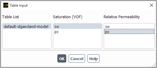
Alternatively, you can specify a user-defined function that calculates the capillary pressure using a
DEFINE_EXCHANGE_PROPERTY macro.
Note: When modeling the capillary pressure, you should ensure that the wetting phases are chosen as the secondary phases.
The following additional field variable is available for secondary phases:
Capillary-Pressure
Note that, although this item is available for both non-wetting and wetting phases, meaningful values are reported only for the wetting phase.
By default, the capillary pressure term is included as a source in the wetting phase momentum equation as shown in Equation 7–22. For two-phase cases, you can use an alternative approach where capillary pressure is modeled as a diffusion term in the wetting phase continuity equation. This approach provides numerical robustness and stability for certain cases.
The gradient of capillary pressure is expressed as a function of the
wetting phase saturation  :
:
 | (7–55) |
The calculation of the gradient of capillary pressure with respect to the wetting phase volume fraction can be done analytically.
To model capillary pressure as diffusion, issue the following text command:
solve/set/multiphase-numerics/porous-media/capillary-pressure-as-diffusion?model capillary pressure as diffusion? [no]yes
Note:
When modeling the capillary pressure as diffusion, the secondary phase must be the wetting phase.
Regardless of whether the flow is laminar or turbulent, Ansys Fluent uses only the viscous resistance in the calculation of capillary pressure gradient.
If you want to include effects of the heat generated by the porous medium in the energy equation, enable the Source Terms option and set a nonzero Energy source. For porous media, energy source terms on the solid and gas sides are applied exactly as entered with no adjustment for porosity. A source term of 100 W/m 3 specified for a solid zone of volume 1.0 m 3 will, therefore, deliver 100 W even if the solids make up only 60% of that volume. You may also define sources of mass, momentum, turbulence, species, or other scalar quantities, as described in Defining Mass, Momentum, Energy, and Other Sources.
If you want to fix the value of one or more variables in the fluid region of the zone, rather than computing them during the calculation, you can do so by enabling the Fixed Values option. See Fixing the Values of Variables for details.
As discussed in Treatment of Turbulence in Porous Media, turbulence will be computed in the porous region just as in the bulk fluid flow. If you are using one of the turbulence models (other than the Large Eddy Simulation model) and you want the turbulence generation to be zero in the porous zone, turn on the Laminar Zone option in the Fluid dialog box. Refer to Specifying a Laminar Zone for more information about suppressing turbulence generation.
Inputs for the rotation axis and zone motion are the same as for a standard fluid zone. See Inputs for Fluid Zones for details.
In general, you can use the standard solution procedures and solution parameter settings when your Ansys Fluent model includes
porous media. You may find, however, that the rate of convergence slows when you define a porous region through which the pressure
drop is relatively large in the flow direction (for example, the permeability,  , is low or the inertial factor,
  , is large). This slow convergence can occur because the porous media pressure drop appears as a momentum source
term—yielding a loss of diagonal dominance—in the matrix of equations solved. The best remedy for poor convergence
of a problem involving a porous medium is to supply a good initial guess for the pressure drop across the medium.
, is large). This slow convergence can occur because the porous media pressure drop appears as a momentum source
term—yielding a loss of diagonal dominance—in the matrix of equations solved. The best remedy for poor convergence
of a problem involving a porous medium is to supply a good initial guess for the pressure drop across the medium.
Similarly, Standard Initialization is the recommended initialization method for porous media simulations. The default Hybrid Initialization method does not account for the porous media properties, and depending on boundary conditions, may produce an unrealistic initial velocity field. For porous media simulations, the Hybrid Initialization method should only be used with the Maintain Constant Velocity Magnitude option.
Another possible way to deal with poor convergence is to temporarily disable the porous media model (by turning off the Porous Zone option in the Fluid Dialog Box) and obtain an initial flow field without the effect of the porous region. With the porous media model turned off, Ansys Fluent will treat the porous zone as a fluid zone and calculate the flow field accordingly. Once an initial solution is obtained, or the calculation is proceeding steadily to convergence, you can enable the porous media model and continue the calculation with the porous region included. (This method is not recommended for porous media with high resistance.)
Simulations involving highly anisotropic porous media may, at times, pose convergence troubles. You can address these issues by
limiting the anisotropy of the porous media coefficients ( and
and  ) to two or three orders of magnitude. Even if the medium’s resistance in one direction is infinite, you
do not need to set the resistance in that direction to be greater than 1000 times the resistance in the primary flow
direction.
) to two or three orders of magnitude. Even if the medium’s resistance in one direction is infinite, you
do not need to set the resistance in that direction to be greater than 1000 times the resistance in the primary flow
direction.
For cases that involve the non-equilibrium thermal model, using a default meshing partitioning method may cause convergence issues and /or solution dependence on the number of processors. In such a case, you should chose a meshing partition method that does not place the partition interface in the regions of significant variations in thermal conductivity and/or mesh size. For more information, see Mesh Partitioning Methods.
The impact of a porous region on the flow field can be determined by examining either velocity components or pressure values. Graphical plots (including report plots of force|lift|drag|moment report definitions— Force and Moment Report Definitions, XY plots— XY Plots of Solution Data , cumulative force/moment plots— Cumulative Force, Moment, and Coefficients Plots, and contour— Displaying Contours and Profiles or vector— Displaying Vectors plots) or alphanumeric reports of the following variables/functions may be of interest:
X, Y, Z Velocity (in the Velocity... category)
Static Pressure (in the Pressure... category)
These variables are contained in the specified categories of the variable selection drop-down list that appears in postprocessing dialog boxes.
Note that thermal reporting in the porous region is defined as follows:
 | (7–56) |
| where | |
 = porosity of the medium = porosity of the medium | |
 = fluid phase thermal conductivity (including the turbulent contribution, = fluid phase thermal conductivity (including the turbulent contribution,  ) ) | |
 = solid medium thermal conductivity = solid medium thermal conductivity |
Important:
Volume and mass integral reports do not account for porosity effects in the porous media.
For porous media involving surface reactions, you can display/report the surface reaction rates using the Arrhenius Rate of Reaction-n in the Reactions... category of the variable selection drop-down list.
Important: Special care must be taken when postprocessing a porous media simulation that utilizes the non-equilibrium thermal model. See Non-Equilibrium Thermal Model for details.
3D fan zones are fluid cell zones that simulate the effect of an axial fan by applying a distributed momentum source in a toroid-shaped fluid volume (that is, a blade-swept volume). This is in contrast to fan boundary conditions (for example, a boundary zone of type fan or intake-fan), which are based on a lumped parameter model in which the fan is considered to be infinitely thin and a discontinuous pressure rise is specified as a function of velocity. 3D fan zones have the following advantages:
3D fan zones can calculate swirl and radial velocities, as opposed to fan boundary conditions, which are mainly used to simulate the axial flow and require you to input swirl and radial coefficients.
The results for 3D fan zones can be comparable to moving reference frame (MRF) simulations, and do not require modeling 3D rotating fan blade geometries.
3D fan zones can simulate a fan even if the available fan curve data was measured at different operating conditions than that of the simulation.
Note: Fluid zones designated as 3D fan zones cannot have non-conformal interfaces.
The following equations are used in the 3D fan zone for the momentum sources in the axial, tangential, and radial directions, which mimic the effect of the fan on the fluid. The tangential momentum source is based on a turbomachinery relation, whereas the radial momentum source is based on a centrifugal force balance.
 | (7–57) |
 | (7–58) |
 | (7–59) |
|
where | |
|
| |
|
| |
|
| |
|
| |
|
| |
|
| |
|
| |
|
| |
|
| |
|
|


In order to calculate the tangential source, three other expressions are necessary:
 | (7–60) |
 | (7–61) |
 | (7–62) |
|
where | |
|
| |
|
| |
|
|


The pressure rise across the 3D fan zone is specified as a function of the volumetric flow rate through the fan. The relationship may be a constant or a fan curve, that is, a polynomial or piecewise-linear function. In the case of a polynomial, the relationship is of the form
 | (7–63) |
where  are the pressure head polynomial coefficients (calculated by Fluent), and
  is the flow rate normal to the fan.
Important: The flow rate  can be either positive or negative. You must be careful to model the fan so that a pressure rise occurs for
forward flow through the fan.
can be either positive or negative. You must be careful to model the fan so that a pressure rise occurs for
forward flow through the fan.
The fan curve data is typically collected at a prescribed set of test conditions. However, the operating conditions of your CFD simulation may be inconsistent with this data (for example, the rotational speed or fluid temperature may be different). To account for this, the 3D fan model can adjust the fan curve data according to the following scaling relationships:
 | (7–64) |
 | (7–65) |
 | (7–66) |
where  and
and  are the test temperature and the volume-averaged temperature of the fan cell zone (which is calculated
internally), respectively.
are the test temperature and the volume-averaged temperature of the fan cell zone (which is calculated
internally), respectively.
A 3D fan zone is modeled as a special type of fluid zone. The cell zone should have a toroid shape that is sized to match the blade-swept volume of the fan you are simulating (that is, has an inner and outer radius that matches the radius of the fan’s hub and blade tips, respectively, as well as a length that matches the thickness of the toroid region swept by the blades in the axial direction). Furthermore, the fluid cell zone should be “interior”, that is, have at least two boundary zones of type interior that border another fluid cell zone and act as the fan inlet and outlet (the other boundaries can be of type interior as well).
To designate a cell zone as a 3D fan zone, enable the 3D Fan Zone option in the Fluid dialog box and then define the geometry and properties of the fan in the 3D Fan Zone tab.
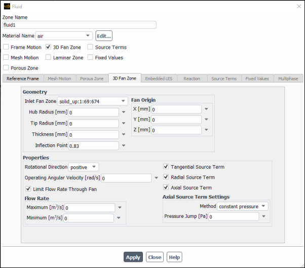
After enabling the 3D Fan Zone option in the Fluid dialog box, you can begin setting it up by defining the settings in the Geometry group box in the 3D Fan Zone tab of the fluid cell zone:
Select a boundary zone from the Inlet Fan Zone drop-down list, which will act as the inlet zone for the 3D fan zone and the surface on which the fan will be located. This boundary must meet certain requirements: it must be of type interior; it must be planar; and it must act as a boundary between the 3D fan zone and another fluid cell zone. Note that the direction the fan blows will be into the 3D fan zone, perpendicular to this boundary zone.
Define the overall dimensions of the fan by entering values for the Hub Radius and the Tip Radius, as well as the Thickness of the toroid region swept by the blades in the axial direction. Note that the values must fit within the confines of the 3D fan zone, and that the Thickness will be applied from the Inlet Fan Zone into the 3D fan zone.
Specify the Inflection Point ratio. The inflection point ratio represents the fraction of the fan blade length (starting at the hub) over which the tangential velocity of the fan discharge is increasing with increasing radius and peaks, before tapering off. See Figure 7.30: The Inflection Point Ratio of a Pitched Blade Turbine for an illustration. You can derive this ratio empirically from experimental data; otherwise, you can first use Ansys Fluent to model the actual fan geometry (for example, using a moving reference frame simulation) and then use those results to determine the input parameters for simpler simulations using the 3D Fan Zone option.
Enter the coordinates for the Fan Origin. This must define a point that is on the plane of the Inlet Fan Zone and located such that the diameters of the fan fall within boundaries of the Inlet Fan Zone.
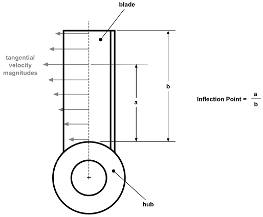
To complete the setup of a 3D fan zone, you must define the settings in the Properties group box in the 3D Fan Zone tab of the fluid cell zone:
Define the Rotational Direction of the fan. The rotation is deemed positive if it follows the right-hand rule with respect to the fan direction vector (that is, a vector from the Fan Origin that points into the 3D fan zone perpendicular to the Inlet Fan Zone).
Specify the Operating Angular Velocity of the fan. This must be a positive nonzero number.
You can enable the Limit Flow Rate Through Fan option, and thereby specify the Maximum and Minimum flow rates that are allowed.
You can enable the Tangential Source Term, Radial Source Term, and/or Axial Source Term options, in order to enable momentum sources in the specified directions. Note that the tangential and radial sources are defined according to impeller theory, and so no further inputs are necessary, whereas the axial source term requires additional input (as described in the step that follows).
If you have enabled the Axial Source Term option, you must define this source in the Axial Source Term Settings group box. For the Method, you can select one of the following choices:
constant pressure
With this method, you must then specify a constant Pressure Jump that is applied to all of the cells in the 3D fan zone.
fan curve
This method allows you to specify the pressure jump through a fan curve (pressure rise vs. volumetric flow rate). Using the Read Fan Curve... button, you can read in a tab-delimited ASCII file that defines the relationship between pressure and flow rate for the 3D fan cell zone (see 3D Fan Curve File Format for details). You must then specify the Curve Fitting Method Fluent should use on the data points in your file, selecting either polynomial or piecewise-linear (for the former, you must then define the Order of Polynomial). Finally, you must provide an estimate of the Initial Flow Rate through your fan zone, as well as the Test Angular Velocity and Test Temperature of the experiment that produced the data points.
Note that a single file can define multiple cell zones, but the file must be read in each of the applicable Fluid dialog boxes.
Note the following limitations when setting up a 3D fan zone:
3D fan zones are not supported with the premixed combustion model.
3D fan zones are not supported with the Eulerian multiphase model.
The Energy Equation must be enabled in the Energy Dialog Box for 3D fan zones when fan curve is selected for the axial source term method.
The option to fix values of variables in Ansys Fluent allows you to set the value of one or more variables in a fluid or solid zone, essentially setting a boundary condition for the variables within the cells of the zone. When a variable is fixed in a given cell, the transport equation for that variable is not solved in the cell (and the cell is not included when the residual sum is computed for that variable). The fixed value is used for the calculation of face fluxes between the cell and its neighbors. The result is a smooth transition between the fixed value of a variable and the values at the neighboring cells.
Important: You can fix values for temperature, species mass fractions, and/or velocity components only if you are using the pressure-based solver. (Refer to Pressure-Based Solver in the Theory Guide for information about the pressure-based solver.)
The ability to fix the value of a variable has a wide range of applications. The velocity fixing method is often used to model the flow in stirred tanks. This approach provides an alternative to the use of a moving reference frame (solution in the reference frame of the blade) and can be used to model baffled tanks. In both 2D and 3D geometries, a fluid cell zone may be used in the impeller regions, and velocity components can be fixed based on measured data.
Although the actual impeller geometry can be modeled and the flow pattern calculated using the sliding mesh model, experimental data for the velocity profile in the outflow region are available for many impeller types. If you do not need to know the details of the flow around the blades for your problem, you can model the impeller by fixing the experimentally-obtained liquid velocities in its outflow zone. The velocities in the rest of the vessel can then be calculated using this fixed velocity profile as a boundary condition. Figure 7.31: Fixing Values for the Flow in a Stirred Tank shows an example of how this method is used to model the flow pattern created by a disk-turbine in an axisymmetric stirred vessel.
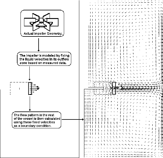
The variables that can be fixed include velocity components (pressure-based solver only), turbulence quantities, temperature (pressure-based solver only), enthalpy, species mass fractions (pressure-based solver only), and user-defined scalars. For turbulence quantities, different values can be set depending on your choice of turbulence model. You can fix the value of the temperature in a fluid or solid zone if you are solving the energy equation. If you are using the non-premixed combustion model, you can fix the enthalpy in a fluid zone. If you have more than one species in your model, you can specify fixed values for the species mass fractions for each individual species except the last one you defined. See the Fluent Customization Manual for details about defining user-defined scalars.
If you are using the Eulerian multiphase model, you can fix the values of velocity components and (depending on which multiphase turbulence model you are using) turbulence quantities on a per-phase basis. See Eulerian Model for details about setting boundary conditions for Eulerian multiphase calculations.
To fix the values of one or more variables in a cell zone, follow these steps (remembering to use only SI units):
In the Fluid Dialog Box or Solid Dialog Box, enable the Fixed Values option.
Fix the values for the appropriate variables in the Fixed Values tab, noting the comments below.
To specify a constant value for a variable, choose constant in the drop-down list next to the relevant field and then enter the constant value in the field.
To specify a non-constant value for a variable, you can use a profile (see Profiles) or a user-defined function for a profile (see the Fluent Customization Manual). Select the appropriate profile or UDF in the drop-down list next to the relevant field.
If you specify a radial-type profile (see Profile Specification Types) for temperature, enthalpy, species mass/mole fractions, or turbulence quantities for the
 -
-  , Spalart-Allmaras, or
  -
-  model, the local coordinate system upon which the radial profile is based is defined by
the Rotation-Axis Origin and Rotation-Axis Direction for the fluid zone.
See Specifying the Rotation Axis for information about setting these parameters. (Note that it is
acceptable to specify the rotation axis and direction for a non-rotating zone. This will not cause the zone to
rotate; it will not rotate unless it has been explicitly defined as a moving zone.)
model, the local coordinate system upon which the radial profile is based is defined by
the Rotation-Axis Origin and Rotation-Axis Direction for the fluid zone.
See Specifying the Rotation Axis for information about setting these parameters. (Note that it is
acceptable to specify the rotation axis and direction for a non-rotating zone. This will not cause the zone to
rotate; it will not rotate unless it has been explicitly defined as a moving zone.)If you do not want to fix the value for a variable, choose (or keep) none in the drop-down list next to the relevant field. This is the default for all variables.
To fix the velocity components, you can specify X, Y, and (in 3D) Z Velocity values, or, for axisymmetric cases, Axial, Radial, and (for axisymmetric swirl) Swirl Velocity values. The units for a fixed velocity are m/s.
For 3D cases, you can choose to specify cylindrical velocity components instead of Cartesian components. Turn on the Local Coordinate System For Fixed Velocities option, and then specify the Axial, Radial, and/or Tangential Velocity values. The local coordinate system is defined by the Rotation-Axis Origin and Rotation-Axis Direction for the fluid zone. See Specifying the Rotation Axis for information about setting these parameters. (Note that it is acceptable to specify the rotation axis and direction for a non-rotating zone. This will not cause the zone to rotate; it will not rotate unless it has been explicitly defined as a moving zone.)
Important: Note the following:
You can fix values for velocity components only if you are using the pressure-based solver. (Refer to Pressure-Based Solver in the Theory Guide for information about the pressure-based solver.)
If all components of velocity are set to fixed values, the solver will also set the gauge pressure to zero on all cells in the cell zone.
If you are solving the energy equation, you can fix the temperature in a zone by specifying the value of the Temperature. The units for a fixed temperature are K.
If you are using the non-premixed combustion model, you can fix the enthalpy in a zone by specifying the value of the Enthalpy. The units for a fixed enthalpy are J/kg.
If you specify a radial-type profile (see Profile Specification Types) for temperature or enthalpy, the local coordinate system upon which the radial profile is based is defined by the Rotation-Axis Origin and Rotation-Axis Direction for the fluid zone. See above for details.
Important: You can fix the value of temperature only if you are using the pressure-based solver.
If you are using the species transport model, you can fix the values of the species mass fractions for individual species. Ansys Fluent allows you to fix the species mass fraction for each species (for example, h2, o2) except the last one you defined.
If you specify a radial-type profile (see Profile Specification Types) for a species mass fraction, the local coordinate system upon which the radial profile is based is defined by the Rotation-Axis Origin and Rotation-Axis Direction for the fluid zone. See above for details.
Important: You can fix values for species mass fractions only if you are using the pressure-based solver.
To fix the values of  and
and  in the
  -
-  equations, specify the Turbulence Kinetic Energy and Turbulence
Dissipation Rate values. The units for
equations, specify the Turbulence Kinetic Energy and Turbulence
Dissipation Rate values. The units for  are
are  /
/ and those for
  are
are  /
/ .
.
To fix the value of the modified turbulent viscosity ( ) for the Spalart-Allmaras model, specify the Modified Turbulent Viscosity value. The
units for the modified turbulent viscosity are
) for the Spalart-Allmaras model, specify the Modified Turbulent Viscosity value. The
units for the modified turbulent viscosity are  /s.
/s.
To fix the values of  and
and  in the
  -
-  equations, specify the Turbulence Kinetic Energy and Specific
Dissipation Rate values. The units for
equations, specify the Turbulence Kinetic Energy and Specific
Dissipation Rate values. The units for  are
are  /
/ and those for
  are 1/s.
To fix the value of  ,
,  , or the Reynolds stresses in the RSM transport equations, specify the Turbulence Kinetic
Energy, Turbulence Dissipation Rate, Specific Dissipation Rate,
UU Reynolds Stress, VV Reynolds Stress, WW Reynolds Stress,
UV Reynolds Stress, VW Reynolds Stress, and/or UW Reynolds
Stress. The units for
, or the Reynolds stresses in the RSM transport equations, specify the Turbulence Kinetic
Energy, Turbulence Dissipation Rate, Specific Dissipation Rate,
UU Reynolds Stress, VV Reynolds Stress, WW Reynolds Stress,
UV Reynolds Stress, VW Reynolds Stress, and/or UW Reynolds
Stress. The units for  and the Reynolds stresses are
  /
/ , and those for
  are
are  /
/ .
.
If you specify a radial-type profile (see Profile Specification Types) for  ,
,  ,
,  , or
, or  , the local coordinate system upon which the radial profile is based is defined by the
Rotation-Axis Origin and Rotation-Axis Direction for the fluid zone. See above for
details. Note that you cannot specify radial-type profiles for the Reynolds stresses.
, the local coordinate system upon which the radial profile is based is defined by the
Rotation-Axis Origin and Rotation-Axis Direction for the fluid zone. See above for
details. Note that you cannot specify radial-type profiles for the Reynolds stresses.
To fix the value of a user-defined scalar, specify the User-defined scalar-n value. (There will be one for each user-defined scalar you have defined.) The units for a user-defined scalar will be the appropriate SI units for the scalar quantity. See the Fluent Customization Manual for information on user-defined scalars.
You can lock (or “freeze”) the temperature values for all the cells in solid zones (including cells to which you have applied an energy source using a UDF) and in walls that have shell conduction enabled, so that the values do not change during further solver iterations. When the temperature is locked for a given cell, the transport equation will still be solved in the cell, and the cell will be included when the residual sum is computed.
You can lock / unlock the temperature for solid and shell zones by using the following text command:
solve → set →
lock-solid-temperature?
Note the following about the option for locking the temperature of solid and shell zones:
It is only available when energy is enabled and the pressure-based solver is selected.
When this option is used, the BCGSTAB option from the Stabilization Method drop-down list of the Advanced Solution Controls dialog box is not supported.
Alternative means of monitoring the convergence of energy may be used.
You can define volumetric sources of mass (for single or multiple species), momentum, energy, turbulence, and other scalar quantities in a fluid zone, or a source of energy for a solid zone. This feature is useful when you want to input a known value for these sources. (For more complicated sources with functional dependency, you can create a user-defined function as described in the separate Fluent Customization Manual.) To add source terms to a cell or group of cells, you must place the cell(s) in a separate zone. The sources are then applied to that cell zone. Typical uses for this feature are listed below:
A flow source that cannot be represented by an inlet, for example, due to an issue of scale. If you need to model an inlet that is smaller than a cell, you can place the cell where the tiny “inlet” is located in its own fluid zone and then define the mass, momentum, and energy sources in that cell zone. For the example shown in Figure 7.32: Defining a Source for a Tiny Inlet, you should set a mass source of
 and a momentum source of
  , where
  is the cell volume.
Heat release due to a source (for example, fire) that is not explicitly defined in your model. For this case, you can place the cell(s) into which the heat is originally released in its own fluid zone and then define the energy source in that cell zone.
An energy source in a solid zone, for conjugate heat transfer applications. For this case, you can place the cell(s) into which the heat is originally released in its own solid zone and then define the energy source in that cell zone.
A species source due to a reaction that is not explicitly included in the model. In the above example of simulating a fire, you might need to define a source for a species representing smoke generation.
Important: Due to the use of the conservative form of the transport equations, when you have a user-specified mass source in the continuity equation, the other equations should have corresponding sources. These secondary sources are not added automatically. You must add them according to the properties (velocity, temperature, mixture composition, and so on) of the added or removed fluid. When specifying such a source for the energy equation, consider the proper definition of the enthalpy value (see The Energy Equation in the Fluent Theory Guide).
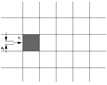
All positive source terms indicate sources, and all negative source terms indicate sinks. All sources must be specified in SI units.
To define one or more source terms for a zone, follow these steps (remembering to use only SI units):
In the Fluid Dialog Box or Solid Dialog Box, turn on the Source Terms option.
Set the appropriate source terms under the Source Terms tab, noting the comments below.
To specify a source, click the button next to the mass, momentum, energy, or other source. The sources dialog box will open where you will define the number of sources. For each source, choose none, constant, or New Input Parameter... in the drop-down list.
If you do not want to specify a source term for a variable, choose (or keep) none in the drop-down list next to the relevant field. This is the default for all variables.
To specify a constant source, choose constant in the drop-down list and then enter the constant value in the field.
To specify a new source parameter, choose New Input Parameter... in the drop-down list and enter the Name or the parameter and the Current Value as a constant.
It is not recommended to only define a mass source without defining the other sources, as described in Defining Mass, Momentum, Energy, and Other Sources above.
Since the sources you specify are defined per unit volume, to determine the appropriate value of your source term you will often need to first determine the volume of the cell(s) in the zone for which you are defining the source. To do this, you can use the Volume Integrals Dialog Box.
In this guide, source is used as a generic term for both source and sink; where source means addition, and sink means subtraction to the physics model. Addition of a source usually leads to the opposite outcome of a sink. For example, a momentum source will accelerate the flow, and in contrast, a momentum sink will decelerate the flow. In general, a source term can be replaced with a sink term with opposite expected outcome.
More details are discussed in the sections that follow.
- 7.2.7.2.1. Mass Sources
- 7.2.7.2.2. Momentum Sources
- 7.2.7.2.3. Energy Sources
- 7.2.7.2.4. Turbulence Sources
- 7.2.7.2.5. Mean Mixture Fraction and Variance Sources
- 7.2.7.2.6. P-1 Radiation Sources
- 7.2.7.2.7. Progress Variable Sources
- 7.2.7.2.8. NO, HCN, and NH3 Sources for the NOx Model
- 7.2.7.2.9. Discrete Bin Fraction Sources for the Population Balance Model
- 7.2.7.2.10. User-Defined Scalar (UDS) Sources
If you have only one species in your problem, you can simply define a
Mass source for that species. The units for the mass source
are  . In the continuity equation (Equation 1–1 in the Theory Guide), the defined mass source will appear in
the
. In the continuity equation (Equation 1–1 in the Theory Guide), the defined mass source will appear in
the  term.
term.
If you have more than one species, you can specify mass sources for each individual species. There will be a total Mass source term as well as a source term listed explicitly for each species (for example, h2, o2) except the last one you defined. If the total of all species mass sources (including the last one) is 0, then you should specify a value of 0 for the Mass source, and also specify the values of the nonzero individual species mass sources. Since you cannot specify the mass source for the last species explicitly, Ansys Fluent will compute it by subtracting the sum of all other species mass sources from the specified total Mass source.
For example, if the mass source for hydrogen in a hydrogen-air mixture is 0.01, the mass source for oxygen is 0.02, and the mass source for nitrogen (the last species) is 0.015, you will specify a value of 0.01 in the h2 field, a value of 0.02 in the o2 field, and a value of 0.045 in the Mass field. This concept also applies within each cell if you use user-defined functions for species mass sources.
The units for the species mass sources are  . In the conservation equation for a chemical species (Equation 7–1 in the Theory Guide), the defined mass
source will appear in the
. In the conservation equation for a chemical species (Equation 7–1 in the Theory Guide), the defined mass
source will appear in the  term.
term.
Note: When a mass source is added in the continuity equation, a corresponding energy source is added in the energy equation at a reference temperature of 0 K for inviscid flows and 298.15 K for viscous flows.
To define a source of momentum, specify the X Momentum,
Y Momentum, and/or Z Momentum term.
The units for the momentum source are N/  . In the momentum equation (Equation 1–3 in the Theory Guide), the defined momentum source will
appear in the
. In the momentum equation (Equation 1–3 in the Theory Guide), the defined momentum source will
appear in the  term.
term.
To define a source of energy, specify an Energy term. The
units for the energy source are W/  . In the energy equation (Equation 5–1 in the Theory Guide), the defined energy source will appear
in the
. In the energy equation (Equation 5–1 in the Theory Guide), the defined energy source will appear
in the  term.
term.
To define a source of  or
or  in the
  -
-  equations, specify the Turbulent Kinetic
Energy or Turbulent Dissipation Rate term.
The units for the
equations, specify the Turbulent Kinetic
Energy or Turbulent Dissipation Rate term.
The units for the  source are kg/m-
  and those for
  are kg/m-
  .
.
The defined  source will appear in the
  term on the right-hand side of the turbulent kinetic
energy equation (for example, Equation 4–39 in the Theory Guide).
term on the right-hand side of the turbulent kinetic
energy equation (for example, Equation 4–39 in the Theory Guide).
The defined  source will appear in the
  term on the right-hand side of the turbulent dissipation
rate equation (for example, Equation 4–40 in the Theory Guide).
term on the right-hand side of the turbulent dissipation
rate equation (for example, Equation 4–40 in the Theory Guide).
To define a source of modified turbulent viscosity, specify the
Modified Turbulent Viscosity term. The units for the
modified turbulent viscosity source are kg/m-  . In the transport equation for the Spalart-Allmaras model
(Equation 4–15 in the Theory Guide), the defined
modified turbulent viscosity source will appear in the
. In the transport equation for the Spalart-Allmaras model
(Equation 4–15 in the Theory Guide), the defined
modified turbulent viscosity source will appear in the  term.
term.
To define a source of  or
or  in the
  -
-  equations, specify the Turbulent Kinetic
Energy or Specific Dissipation Rate term.
The units for the
equations, specify the Turbulent Kinetic
Energy or Specific Dissipation Rate term.
The units for the  source are kg/m-
  and those for
  are kg/
  -
-  .
.
The defined  source will appear in the
  term on the right-hand side of the turbulent kinetic
energy equation (Equation 4–71 in the Theory
Guide).
term on the right-hand side of the turbulent kinetic
energy equation (Equation 4–71 in the Theory
Guide).
The defined  source will appear in the
  term on the right-hand side of the specific turbulent
dissipation rate equation (Equation 4–72 in the Theory Guide).
term on the right-hand side of the specific turbulent
dissipation rate equation (Equation 4–72 in the Theory Guide).
To define a source of  ,
,  , or the Reynolds stresses in the RSM transport equations,
specify the Turbulence Kinetic Energy,
Turbulence Dissipation Rate, Specific
Dissipation Rate, UU Reynolds Stress,
VV Reynolds Stress, WW Reynolds
Stress, UV Reynolds Stress, VW
Reynolds Stress, and/or UW Reynolds Stress
terms. The units for the
, or the Reynolds stresses in the RSM transport equations,
specify the Turbulence Kinetic Energy,
Turbulence Dissipation Rate, Specific
Dissipation Rate, UU Reynolds Stress,
VV Reynolds Stress, WW Reynolds
Stress, UV Reynolds Stress, VW
Reynolds Stress, and/or UW Reynolds Stress
terms. The units for the  source and the sources of Reynolds stress are kg/m-
 , and those for
  are kg/m-
  .
.
The defined Reynolds stress sources will appear in the  term on the right-hand side of the Reynolds stress
transport equation (Equation 4–226 in the Theory Guide).
term on the right-hand side of the Reynolds stress
transport equation (Equation 4–226 in the Theory Guide).
The defined  source will appear in the
  term on the right-hand side of Equation 4–254 in the Theory Guide.
The defined  will appear in the
  term on the right-hand side of Equation 4–257 in the Theory Guide.
To define a source of the mean mixture fraction or its variance for the
non-premixed combustion model, specify the Mean Mixture
Fraction or Mixture Fraction Variance term. The
units for the mean mixture fraction source are  , and those for the mixture fraction variance source are
 .
.
The defined mean mixture fraction source will appear in the  term in the transport equation for the mixture fraction
(Equation 8–4 in the Theory Guide).
term in the transport equation for the mixture fraction
(Equation 8–4 in the Theory Guide).
The defined mixture fraction variance source will appear in the
 term in the transport equation for the mixture fraction
variance (Equation 8–5 in
the Theory Guide).
term in the transport equation for the mixture fraction
variance (Equation 8–5 in
the Theory Guide).
If you are using the two-mixture-fraction approach, you can also specify sources of the Secondary Mean Mixture Fraction and Secondary Mixture Fraction Variance.
To define a source for the P-1 radiation model, specify the
P1 term. The units for the radiation source are W/
 , and the defined source will appear in the
  term in Equation 5–57
in the Theory Guide.
term in Equation 5–57
in the Theory Guide.
Note that, if the source term you are defining represents a transfer from internal energy to radiative energy (for example, absorption or emission), you must specify an Energy source of the same magnitude as the P1 source, but with the opposite sign, in order to ensure overall energy conservation.
To define a source of the progress variable for the premixed combustion model,
specify the Progress Variable term. The units for the
progress variable source are kg/  -s, and the defined source will appear in the
  term in Equation 8–70 in the Theory Guide.
To define a source of NO, HCN, or  for the NOx model, specify the no,
hcn, or nh3 term. The units for these
sources are kg/
for the NOx model, specify the no,
hcn, or nh3 term. The units for these
sources are kg/  -s, and the defined sources will appear in the
  ,
,  , and
, and  terms of Equation 9–1, Equation 9–2, and Equation 9–3 in the Theory Guide.
For the Discrete and Inhomogeneous
Discrete population balance models, you can specify
Bin-i-fraction source terms
(where i is the bin label). Note that bins are
labeled from 0 to  , where
  is the number of bins that you specified in the
Population Balance Model tab of the Multiphase
Model dialog box. The units for the fraction source are
kg/m3 s.
is the number of bins that you specified in the
Population Balance Model tab of the Multiphase
Model dialog box. The units for the fraction source are
kg/m3 s.
You can specify source term(s) for each UDS transport equation you have defined in your model. See Setting Up UDS Equations in Ansys Fluent for details.