


Experiments in roughened pipes and channels indicate that the mean velocity distribution
near rough walls, when plotted in the usual semi-logarithmic scale, has the same slope
( ) but a different intercept (additive constant
  in the log-law). Therefore, the law-of-the-wall for mean velocity modified for
roughness has the form
in the log-law). Therefore, the law-of-the-wall for mean velocity modified for
roughness has the form
 | (4–412) |
where  and
and
 | (4–413) |
where  is a roughness function that quantifies the shift of the intercept due to
roughness effects.
is a roughness function that quantifies the shift of the intercept due to
roughness effects.
For  -based wall functions for LES (see Harmonic Blending Wall Functions Based on r+), the
logarithmic part of the profile is shifted at rough walls using following formulation:
-based wall functions for LES (see Harmonic Blending Wall Functions Based on r+), the
logarithmic part of the profile is shifted at rough walls using following formulation:
 | (4–414) |
 depends, in general, on the type (uniform sand, rivets, threads, ribs,
mesh-wire, and so on) and size of the roughness. There is no universal roughness function valid
for all types of roughness. For a sand-grain roughness and similar types of uniform roughness
elements, however,
depends, in general, on the type (uniform sand, rivets, threads, ribs,
mesh-wire, and so on) and size of the roughness. There is no universal roughness function valid
for all types of roughness. For a sand-grain roughness and similar types of uniform roughness
elements, however,  has been found to be well-correlated with the nondimensional roughness height,
 , where
  is the physical roughness height and
  . Analyses of experimental data show that the roughness function is not a single
function of
. Analyses of experimental data show that the roughness function is not a single
function of  , but takes different forms depending on the
  value. It has been observed that there are three distinct regimes:
hydrodynamically smooth (
 )
)transitional (
 )
)fully rough (
 )
)
According to the data, roughness effects are negligible in the hydrodynamically smooth regime, but become increasingly important in the transitional regime, and take full effect in the fully rough regime.
In Ansys Fluent, the whole roughness regime is subdivided into the three regimes, and the
formulas proposed by Cebeci and Bradshaw based on Nikuradse’s data [98] are adopted to compute  for each regime.
For the hydrodynamically smooth regime ( ):
):
 | (4–415) |
For the transitional regime ( ):
):
 | (4–416) |
where  is a roughness constant, and depends on the type of the roughness.
In the fully rough regime ( ):
):
 | (4–417) |
In the solver, given the roughness parameters,  is evaluated using the corresponding formula (Equation 4–415, Equation 4–416, or Equation 4–417). The modified law-of-the-wall in Equation 4–412 is then used to evaluate the shear stress at the wall and
other wall functions for the mean temperature and turbulent quantities.
is evaluated using the corresponding formula (Equation 4–415, Equation 4–416, or Equation 4–417). The modified law-of-the-wall in Equation 4–412 is then used to evaluate the shear stress at the wall and
other wall functions for the mean temperature and turbulent quantities.
 represents a downward shift of the logarithmic velocity profile, as shown in
the following figure:
represents a downward shift of the logarithmic velocity profile, as shown in
the following figure:
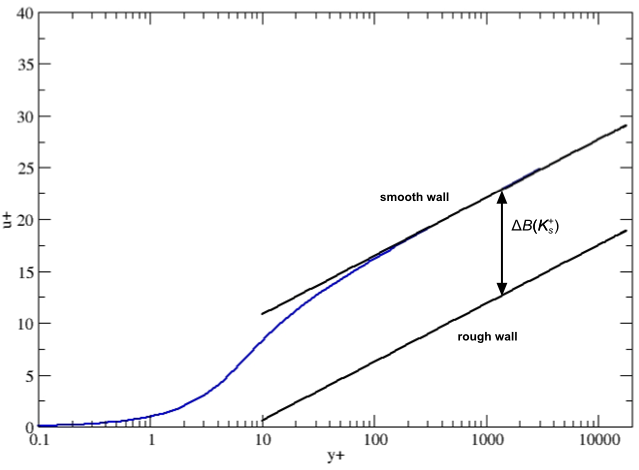
This downward shift leads to a singularity for large roughness heights and low values of
 . Depending on the turbulence model and near wall treatment, two different
approaches are used in Ansys Fluent in order to avoid this issue:
. Depending on the turbulence model and near wall treatment, two different
approaches are used in Ansys Fluent in order to avoid this issue:
reducing the roughness height as
 decreases
The first approach consists in redefining the roughness height based on the mesh refinement:

(4–418)
This ensures that as
 approaches zero, so too does
  . Therefore, the mesh requirement for rough walls in this case is
 , in order to maintain the full effect of the roughness on the flow.
virtually shifting the wall
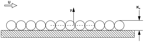
The second approach is based on the observation that the viscous sublayer is fully established only near hydraulically smooth walls. In the transitional roughness regime, the roughness elements are slightly thicker than the viscous sublayer and start to disturb it, so that in fully rough flows, the sublayer is destroyed and viscous effects become negligible. The following figure illustrates the equivalent sand-grain roughness using a wall with a layer of closely packed spheres, which have an average roughness height representing a technical roughness with peaks and valleys of different shapes and sizes (see Schlichting and Gersten [578]):
It can be assumed that the roughness has a blockage effect, which is about 50% of its height (note that the figure above shows a two-dimensional cut of a three-dimensional arrangement).
It is therefore sensible to virtually shift the wall to 50% of the height of the roughness elements. This results in a corrected
 value for the first cell center:
(4–419)
which gives about the correct displacement caused by the surface roughness. Thus the singularity issue is avoided and fine meshes can be handled correctly.
The second approach (that is, virtually shifting the wall) is the default treatment for
rough walls for all two-equation turbulence models based on the  -equation and for the following turbulence models based on the
  -equation, when they are used with standard and scalable wall functions (note
that the use of scalable wall functions is recommended over the use of standard wall
functions):
-equation, when they are used with standard and scalable wall functions (note
that the use of scalable wall functions is recommended over the use of standard wall
functions):
standard, RNG, and realizable
 -
-  model
modelReynolds stress models
All other model combinations with rough walls (for example, the Spalart-Allmaras model and
LES in combination with Harmonic Blending Wall Functions Based on r+) have no special calibration on
fine meshes, and therefore the first approach (reducing the roughness height as  decreases) is used.
Note: The advantage of the rough wall formulation using a virtual shift of the wall (Equation 4–419) compared to reducing the roughness height as
decreases (Equation 4–418) is that it
eliminates all restrictions with respect to mesh resolution near the wall, and can therefore be
used on arbitrarily fine meshes.
Important: Prior to Ansys Fluent 14, the shift described by Equation 4–419 was not applied when using turbulence models based
on the  -equation. You can recover the previous code behavior by using the following
scheme command:
-equation. You can recover the previous code behavior by using the following
scheme command:
(rpsetvar 'ke-rough-wall-treatment-r14? #f)
(models-changed)