28.2. Setting Up an Intrinsic Fluid-Structure Interaction (FSI) Simulation

The procedure for setting up an intrinsic FSI simulation is described below. Note that only steps that are pertinent to the structural model are listed here. You will also need to define the other settings (such as other material properties, boundary conditions, other models) as usual. For information about inputs related to other Ansys Fluent models that you are using in conjunction with the intrinsic FSI simulation, refer to the appropriate sections for those models.

Important: Double Precision is recommended for all intrinsic FSI simulations.

Define the settings in the General task page.
Setup → General
1. Define the time dependence of the simulation: one-way FSI problems can be Steady or Transient, whereas two-way FSI problems must be Transient. Note that modeling two-way FSI is only necessary when the deformation of the solid zone is significant enough to affect the fluid flow.
2. You can enable the Gravity option and define the coordinates for the acceleration if you would like the structural model to account for gravitational forces when calculating the deformation of the solid cell zone.
Define a solid zone.
Setup → Cell Zone Conditions
Note that you can enable the Frame Motion option in the Solid dialog box and define a rotational velocity for the reference frame if you would like the structural model to account for rotational forces when calculating the deformation of the solid cell zone. For details, see Defining Zone Motion and Modeling Flows with Moving Reference Frames.
For a two-way FSI problem, it is recommended that you run the calculation at this point to obtain a converged solution for the fluid, and then proceed with the following steps to set up and run the structural model.
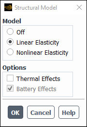
In the Structural Model dialog box, select a variation of the structural model.
- The Linear Elasticity model enables structural calculations for the solid cell zone such that the internal load is linearly proportional to the nodal displacement, and the structural stiffness matrix remains constant.
- The Nonlinear Elasticity model allows you to model geometrically nonlinear elasticity, in order to simulate large deformation in solid cell zones.
- The structural model allows you to model linear or nonlinear thermo-elasticity, in order to simulate the effects of thermal load on solid structure deformation. To set up such a simulation, choose the Thermal Effects option in the Structural Model dialog box.
  Thermoelasticity also can be enabled via the text user interface using the following command:
  define → models → structure → controls → thermal-effects?
  Note that thermal effects are only available for the linear or nonlinear structural model if the energy equation is enabled.
- For Newman’s P2D battery cases that include swelling effects, you can model linear or nonlinear elasticity (see Inputs for the Newman’s P2D Model). After selecting an elasticity model in the Structural Model dialog box, the Battery Effects option is enabled automatically and cannot be disabled.
Setup → Models → Structure Edit...
Figure 28.1: The Structural Model Dialog Box
Make sure that the material used in the solid cell zone is properly defined, by setting the Youngs Modulus and Poisson Ratio fields in the Properties group box of the Create/Edit Materials dialog box.
Setup → Materials
Thermo-elasticity requires you to set up two additional parameters per solid material used:
- Starting Temperature [K]
  The starting temperature specified in the Materials dialog box will be constant by default. If your problem requires a non-constant starting temperature for thermo-elastic analysis, the following procedure is recommended:
  1. First perform an initial calculation to solve for the temperature field within the solid zones of your problem (for more information see Modeling Conductive and Convective Heat Transfer).
  2. Re-assign the temperature field calculated in the previous step as the non-constant starting temperature, by entering the following TUI command in the console:
    /define/models/structure/expert/starting-t-re-initialization?
    When prompted with Starting T-field re-initialization method (0 1) [0], enter 1. This will perform re-initialization of the new starting temperature field for structural analysis.
    The new starting temperature field can be visualized by displaying contours of Structure and Starting Structure Temperature within the Contours Dialog Box.
    Note that after re-initializing the starting temperature field, the starting temperature will no longer be available within the Materials dialog box.
- Thermal Expansion [1/K]
Note that the Youngs Modulus, Poisson Ratio, and Thermal Expansion can also be defined using a user-defined function (UDF) by interpreting or compiling a suitable UDF. For details, see DEFINE_PROPERTY UDFs.
If you plan to define volumetric body force as a source term for a solid cell zone using a user-defined function (UDF), interpret or compile a suitable UDF. For details, see DEFINE_SOURCE_FE.
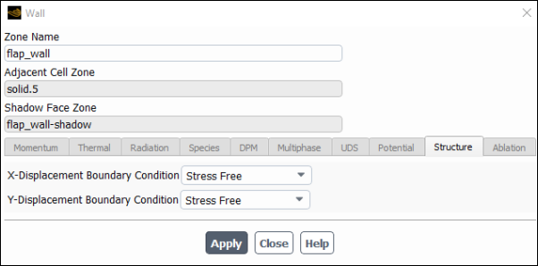
If you plan to define the displacement or force applied to the nodes of a wall adjacent to the solid zone using a user-defined function (UDF), interpret or compile a suitable UDF. For details, see DEFINE_WALL_NODAL_DISP or DEFINE_WALL_NODAL_FORCE, respectively.
For every wall that is immediately adjacent to the solid zone, define the displacement boundary condition settings in the Structure tab of the Wall dialog box.
Setup → Boundary Conditions
Figure 28.2: The Structure Tab of the Wall Dialog Box

The walls will be one-sided when they are only adjacent to a solid cell zone, and will be two-sided (that is, a wall / wall-shadow pair) when they are adjacent to both a solid and a fluid cell zone. Note that for two-sided walls, the Structure tab is only available for one side of the wall / wall-shadow pair; which one will depend on how the mesh was set up.
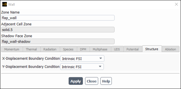
You must select one of the following from the X-, Y-, and (for 3D cases) Z-Displacement Boundary Condition drop-down lists, in order to define how the displacement is calculated for the nodes in that particular direction:
- Stress Free specifies that the displacement is not affected by stress loads from the fluid flow.
- Node X-, Node Y-, and (for 3D cases) Node Z-Force specifies that the displacement results from a specified force applied on the nodes, which is defined using the Node X-, Node Y-, and (for 3D cases) Node Z-Force field.
- Node X-, Node Y-, and (for 3D cases) Node Z-Displacement applies a specified displacement on the nodes, which is defined using the X-, Y-, and (for 3D cases) Z-Displacement field.
- Face Pressure specifies that the displacement results from a specified pressure load applied on the faces, which is defined using the Face Pressure field.
- Intrinsic FSI specifies that the displacement results from pressure loads exerted by the fluid flow on the faces. Note that this selection is only available for a zone that is part of a wall / wall-shadow pair.
Note: You can specify the nodal force (Node X-Force, Node Y-Force and Node Z-Force), displacement (Node X-Displacement, Node Y-Displacement and Node Z-Displacement) as well as the Face Pressure using a constant value, an input parameter, an interpreted or compiled user-defined function (see DEFINE_WALL_NODAL_DISP or DEFINE_WALL_NODAL_FORCE in the Fluent Customization Manual), or you can use an expression (see Fluent Expressions Language).
Figure 28.3: The Wall Dialog Box for a Two-Sided Wall

In a typical Fluent simulation, symmetry boundary conditions are used for boundaries on the solid zone and the same strategy can be applied for intrinsic FSI Fluent simulations. Alternatively, the plane of symmetry, when aligned with Cartesian planes, could be modeled using a wall boundary condition. For example, when the symmetry plane is the XY plane, you should assign the x- and y-displacement to Stress Free and then assign the z-displacement to 0
Note: When solving a structural problem, boundary conditions that allow for structural rigid body motion can lead to an ill-posed problem. That is, if it is at all possible that any motion can lead to a scenario with no stresses, then the problem cannot be solved. Fluent can analyze the setup and will provide a warning when such motion is not prevented by boundary conditions (except when disconnected regions belong to a single solid zone). Such problematic configurations should therefore be avoided.
For two-way FSI simulations, define dynamic mesh properties to allow the mesh to handle the deformation of the solid zone. This includes the following:
- Enable dynamic mesh Smoothing, and select either the Diffusion, Linearly Elastic Solid, or Radial Basis Function method in the Mesh Method Settings Dialog Box.
- For cases with strong FSI coupling (such as when the fluid and solid densities are comparable or for large deformations), enable the Implicit Update option in the Dynamic Mesh task page and define appropriate settings in the Implicit Update tab of the Options dialog box. For details, see Setting Dynamic Mesh Modeling Parameters and Implicit Update Settings.
- Define an Intrinsic FSI dynamic mesh zone for the side of a two-sided wall (that is, the wall or wall-shadow) that is immediately adjacent to the fluid cell zone (as indicated by the Adjacent Cell Zone field in the Wall dialog box). For further details, see Intrinsic FSI Motion. You should create stationary dynamic mesh zones for all the boundaries that are not deforming.
Setup → Dynamic Mesh
For transient simulations, you can make a selection from the Structure Transient Formulation drop-down list in the Solution Methods Task Page to specify the direct time integration method used to solve the finite element semi-discrete equation of motion. You can select from the Newmark method (default) or the Backward Euler method. For further details about these methods, see Dynamic Structural Systems in the Theory Guide.
Solution → Methods
You can revise the following settings if you find that the defaults do not produce satisfactory results:
- You can specify the solution method used by the linear solver for the structural model calculations. By default, the bi-conjugate gradient stabilized (BCGSTAB) method is used. This method offers a good balance of speed and robustness. If divergence is detected with BCGSTAB, then the generalized minimal residual (GMRES) method will be used for an iteration as a fallback, and you will be informed in the console that a "fe-structure" equation is being stabilized to enhance linear solver robustness. If you find that your residual level / drop is not satisfactory, you can try increasing the maximum number of inner iterations from the default of 500 by using the following text command:
  define → models → structure → controls → max-iter
  If the BCGSTAB method continues to produce unsatisfactory residuals with a higher number of inner iterations or if you repeatedly see console messages that say the GMRES fallback is being used, you can change the solution to the GMRES method. Note that GMRES is the most robust method, but it is also more demanding in terms of memory usage and solver time. With GMRES, it is recommended that you start with the maximum iterations set to 50. Also available is the conjugate gradient (CG) method: while in some cases it is the least robust method, it can result in faster calculations, as it takes advantage of the symmetry of the matrix used in the linear systems of equations. To change the solution method, use the following text command:
  define → models → structure → controls → amg-stabilization
- For transient simulations, you can revise the numerical damping factor for the structural model calculations (that is, the amplitude decay factor in Equation 16–16 in the Theory Guide) by using the following text command:
  define → models → structure → controls → numerical-damping-factor?
- You can enable an explicit fluid-structure interaction force by using the following text command:
  define → models → structure → expert → explicit-fsi-force?
- You can enable the inclusion of operating pressure into the fluid-structure interaction force by using the following text command:
  define → models → structure → expert → include-pop-in-fsi-force?
- You can enable the inclusion of a viscous fluid-structure interaction force by using the following text command:
  define → models → structure → expert → include-viscous-fsi-force?
- When the deformation of a structure is mainly due to bending, the displacement can be underestimated when a linear interpolation is used for the displacement, especially on rather coarse meshes. This is often referred to as shear locking, as the representation of the bending requires the shearing of linear elements which actually absorbs a part of the energy put into the bending.
  The effects of shear locking can be corrected by invoking the enhanced strain element. It is available for quad cells in 2D and hex cells in 3D.
  The enhanced strain element can be enabled in the TUI using the command:
  define → models → structure → controls → enhanced-strain?
  and by subsequently answering yes at the prompt.
- To enable Rayleigh damping for unsteady simulations (Rayleigh Damping), enter the following text user interface (TUI) command:
  define → models → structure → controls → unsteady-damping-rayleigh?
  The following damping coefficients are available for solid materials:
  - Mass Proportional Damping [1/s]
  - Stiffness Proportional Damping [s]
If necessary, revise the default convergence criteria for the x- y-, and (for 3D cases) z-displacement residual equations in the Residual Monitors Dialog Box.
Solution → Monitors → Residual Edit...
(Optional) Create structural point surfaces at points of interest within the solid zone, which you can use for monitoring and reporting data. Note that for two-way FSI simulations, a structural point surface does not necessarily remain fixed in space, but will continue to represent its original cell as the solid zone moves / deforms.
Results → Surfaces New → Structural Point...
For further details, see Structural Point Surfaces.
To monitor a field variable at such a structural point surface, create a report definition. For example, you could monitor and plot the vertex average of the displacement of the nodes that surround a structural point surface:
Solution → Report Definitions New → Surface Report → Vertex Average...
For further details, see Creating Report Definitions.
Initialize the solution. Note that for standard initialization, you can specify the initial X, Y, and (for 3D cases) Z Displacement in the Solution Initialization Task Page.
Solution → Initialization
Note: In order to ensure the quality for structural model files, only the Common Fluids Format (CFF) is supported when writing case and data files when the structural model is enabled.
(Optional) For two-way FSI simulations, set up solution animations.
You can capture results for the transient simulation as it calculates the solution and then later display how the fluid flow and/or the solid shape (node displacement and/or mesh) changes over time. You should narrow the min-max range, since the contour changes may be small. See Animating Graphics for more information.
Results → Animations → Scene Animation Edit...
Run the calculation.
Solution → Run Calculation
Tip: For one-way FSI simulations, the calculation time will be faster if you first run the calculation with only the fluid equations enabled in the Equations dialog box, and then run it with only the structure equation enabled.
Solution → Controls Equations...
For one-way or two-way FSI, it is also recommended that you solve the steady flow problem first, because it allows you to easily discern and resolve any convergence issues that are not related to the fluid-structure interaction.
View the results by displaying contours of the following field variables (in the Structure... category, also available for displaying vectors):
- Total Displacement
- X, Y, and Z Displacement for the displacement values
- Sigma XX, YY, XY, ZZ, YZ, and XZ for the stress tensor values
- von Mises Stress for material failure analysis (being automatically calculated once selected here for postprocessing)
Results → Graphics → Contours New...
Note:
- You should confirm that the stress loading does not exceed the yield strength of the solid material, as this is an assumption of the Linear Elasticity structural model.
- While contours of the Structures... field variables are only displayed in solid cell zones, a few displays do not follow this paradigm: contours based on expressions or custom field functions, minimum/maximum computations, and XY plots.

28.2.1. Using Intrinsic FSI With Non-Conformal Interfaces

In many FSI applications, meshes for solid zones are prepared differently from fluid zones. Typically, the mesh quality for a finite element analysis is not as critical as the mesh quality for a computational fluid dynamics analysis. Since it is common to have a non-conformal mesh at the fluid-solid interface, support for non-conformal interfaces for one-way and two-way FSI calculations is desirable.

Note: It is assumed that the mesh for the solid side surface can be either quadrilateral or triangular in 3D, and that ANSYS Fluent calculates the intersection facets (that is, the faces imprinted from, and interested with, the other surface) at the non-conformal interface.

Note: Solid-solid non-conformal interfaces are not supported; only fluid-solid interfaces are supported.

To use non-conformal interfaces in your intrinsic FSI simulation, perform the following steps:

Read your mesh into an Ansys Fluent session.
Create your mesh interface(s).
Setup → Mesh Interfaces New...
Enable the Structural Model.
Setup → Models → Structure Edit...
Choose the appropriate intrinsic FSI structural model (Linear or Nonlinear)
Set up the intrinsic FSI boundary condition and dynamic mesh settings.
Setup → Boundary Conditions
Setup → Dynamic Mesh
Define intrinsic FSI boundary condition and dynamic mesh settings on those wall boundaries that were automatically created as part of defining the mesh interface(s).
Set up the rest of the intrinsic FSI problem as you normally would, as described in Setting Up an Intrinsic Fluid-Structure Interaction (FSI) Simulation.