Many problems permit the entire computational domain to be referred to a single moving reference frame (hence the name SRF modeling). In such cases, the equations given in Equations for a Moving Reference Frame are solved in all fluid cell zones. Steady-state solutions are possible in SRF models provided suitable boundary conditions are prescribed. In particular, wall boundaries must adhere to the following requirements:
Any walls that are moving with the reference frame can assume any shape. An example would be the blade surfaces associated with a pump impeller. The no slip condition is defined in the relative frame such that the relative velocity is zero on the moving walls.
For a rotating problem, you can define walls that are non-moving with respect to the stationary coordinate system, but these walls must be surfaces of revolution about the axis of rotation. Here the no slip condition is defined such that the absolute velocity is zero on the walls. An example of this type of boundary would be a cylindrical wind tunnel wall that surrounds a rotating propeller.
Rotationally periodic boundaries may also be used, but the surface must be periodic about the axis of rotation. As an example, it is very common to model flow through a blade row of a turbomachine by assuming the flow to be rotationally periodic and using a periodic domain about a single blade. This permits good resolution of the flow around the blade without the expense of modeling all blades in the blade row (see Figure 10.3: Single Blade Model with Rotationally Periodic Boundaries).
Flow boundary conditions in Ansys Fluent (inlets and outlets) can, in most cases, be prescribed in either the stationary or moving frames. For example, for a velocity inlet, one can specify either the relative velocity or absolute velocity, depending on which is more convenient. For additional information on these and other boundary conditions, see Setting Up a Single Moving Reference Frame Problem and Cell Zone and Boundary Conditions.
It is important to remember the following coordinate-system constraints when you are setting up a problem involving a moving reference frame for a rotating problem:
For 2D problems, the axis of rotation must be parallel to the
 axis.
axis.For 2D axisymmetric problems, the axis of rotation must be the
 axis.
axis.For 3D geometries, you should generate the mesh with a specific origin and rotational axis in mind for the rotating cell zone. Usually it is convenient to use the origin of the global coordinate system (0,0,0) for the frame origin, and either the
 ,
,  , or
, or  axis for the rotational axis;
however, Ansys Fluent can accommodate an arbitrary origin and rotational
axis.
axis for the rotational axis;
however, Ansys Fluent can accommodate an arbitrary origin and rotational
axis.
With 3D rotating problems, it is also important to note that if you want to include walls that have zero velocity in the stationary frame, these walls must be a surface of revolution with respect to the axis of rotation. If the stationary walls are not surfaces of revolution, you must encapsulate the rotating parts with interface boundaries, thereby breaking your model up into multiple zones, and use the MRF model for a steady-state solution (see The Multiple Reference Frame Model), or the sliding mesh model for unsteady interaction (see Modeling Flows Using Sliding and Dynamic Meshes).
To model a problem involving a single moving reference frame, follow the steps outlined below.
Select the Velocity Formulation to be used when solving: either Relative or Absolute. (See Choosing the Relative or Absolute Velocity Formulation for details.)
 Setup →
  General
(Note that this step is irrelevant if you are using one of the density-based solvers; these solvers always use an absolute velocity formulation.)
For each cell zone in the domain, specify the translational velocity of the reference frame and/or the angular velocity (
 ) of the reference frame and the axis about which it rotates. Setup → Cell Zone
Conditions
) of the reference frame and the axis about which it rotates. Setup → Cell Zone
Conditions
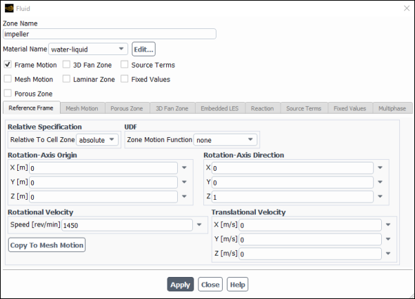
In the Fluid or Solid dialog box, specify the Rotation-Axis Origin and Rotation-Axis Direction for the frame motion in the Reference Frame tab, in order to define the axis of rotation.
Also in the Fluid (Figure 10.4: The Fluid Dialog Box Displaying Frame Motion Inputs) or Solid dialog box, enable the Frame Motion option. (Note that a solid zone cannot move at a different speed than an adjacent solid zone; for such a situation, you must instead use Solid Motion.)
In the Reference Frame tab, set the Speed under Rotational Velocity and/or the X, Y, and Z components of the Translational Velocity. Note that the speed can be specified as a constant value or a transient profile. The transient profile may be in a file format, as described in Transient Cell Zone and Boundary Conditions, or a UDF macro, described in
DEFINE_TRANSIENT_PROFILE. Specifying the individual velocities as either a profile or a UDF allows you to specify a specific input of the frame motion individually. However, you can also specify the frame motion inputs via a single user-defined function that uses the UDF macroDEFINE_ZONE_MOTION. This may prove to be quite convenient if you are modeling a more complicated motion of the moving reference frame, where the hooking of many different user-defined functions or profiles can be cumbersome.Note: If you decide to hook a UDF, you will no longer have access to the rotation axis origin and direction, or the velocities.
Details about these inputs are presented in Inputs for Fluid Zones and in Inputs for Solid Zones. Details about the zone motion UDF can be found in
DEFINE_ZONE_MOTIONin the Fluent Customization Manual.If you need to switch between the moving reference frame and moving mesh models, simply click the Copy To Mesh Motion for zones with a moving frame of reference and Copy to Frame Motion for zones with moving meshes to transfer motion variables, such as the axes, frame origin, and velocity components between the two models. The variables used for the origin, axis, and velocity components, as well as for the UDF
DEFINE_ZONE_MOTIONwill be copied. This is particularly useful if you are doing a steady-state MRF simulation to obtain an initial solution for a transient Moving Mesh simulation in a turbomachine.
Important: Normally it is not necessary to enable the Frame Motion option for solid zones, as this is not required if you want to do a conjugate heat transfer problem where the solid and fluid zones are moving together. A case in which you would want to enable the Frame Motion option is if you are running an intrinsic fluid-structure-interaction (FSI) simulation, and you want the structural model to account for rotational forces when calculating the deformation of the solid cell zone (see Modeling Fluid-Structure Interaction (FSI) Within Fluent).
Define the velocity boundary conditions at walls. You can choose to define either an absolute velocity or a velocity relative to the moving reference frame (that is, relative to the velocity of the adjacent cell zone specified in step 2).
If the wall is moving at the speed of the moving frame (and hence stationary in the moving frame), it is convenient to specify a relative angular velocity of zero. Likewise, a wall that is stationary in the non-moving frame of reference should be given a velocity of zero in the absolute reference frame. Specifying the wall velocities in this manner obviates the need to modify these inputs later if a change is made in the velocity of the fluid zone.
Details about these inputs are presented in Velocity Conditions for Moving Walls.
Define the boundary conditions at the inlets, as described in Boundary Conditions. For velocity inlets, you can choose to define either absolute velocities or velocities relative to the motion of the adjacent cell zone (specified in step 2). Likewise, the total pressure and flow direction can be prescribed in absolute or relative frames for pressure inlets.
Details about these inputs are presented in Defining the Flow Direction and Defining the Velocity.
(optional) For transient cases, after you have initialized or run the calculation you can use the Moving Mesh Courant Number field variable (in the Velocity... category) to guide your solution. This field variable is a non-dimensional value that indicates the number of cells that might be swept in a single time step due to a mesh motion.
It is recommended that you use the velocity formulation that will result in most of the flow domain having the smallest velocities in that frame, thereby reducing the numerical diffusion in the solution and leading to a more accurate solution.
The absolute velocity formulation is preferred in applications where the flow in most of the domain is not moving (for example, a fan in a large room). The relative velocity formulation is appropriate when most of the fluid in the domain is moving, as in the case of a large impeller in a mixing tank.
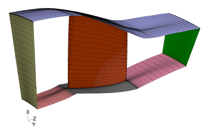
A problem with stationary outer walls and a rotating impeller can be solved in a single reference frame. The example is illustrated in Figure 10.5: Geometry with the Rotating Impeller.
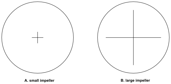
In case A, it is expected that only the flow near the impeller would be rotating and that much of the flow away from the impeller would have a low velocity magnitude in the absolute frame. Therefore, solving using the absolute velocity formulation is recommended. In case B, most of the flow is expected to be rotating with a velocity close to that of the impeller. Hence, the relative velocity formulation is appropriate.
In a situation between case A and case B, either of the formulations may be used.
Important:
If the velocity formulation is switched during the solution process, Ansys Fluent will not transform the current solution to the other frame, which can lead to large jumps in residuals. If changing the frame is necessary, it is recommended that you first reinitialize, and then solve.
When one of the density-based solution algorithms is used, the absolute formulation is always used; the relative velocity formulation is not available in the density-based solvers.
For velocity inlets, pressure inlets, mass-flow inlets, and walls, you may specify velocity in either the absolute or the relative frame, regardless of whether the absolute or relative velocity formulation is used in the computation. Note, that the inlet turbulence values are processed using the velocity values, which are converted to the Velocity Formulation selected in the General Task Page, see explanations in Estimating Turbulent Kinetic Energy from Turbulence Intensity and in the introductory part of Inlet Boundary Conditions for Scale Resolving Simulations.
For pressure outlets, the specified static pressure is independent of frame. However, when there is backflow at a pressure outlet, the specified static pressure is used as the total pressure. For calculations using the absolute velocity formulation, the specified static pressure is used as the total pressure in the absolute frame; for the relative velocity formulation, the specified static pressure is assumed to be the total pressure in the relative frame. As for the flow direction, Ansys Fluent assumes the absolute velocity to be normal to the pressure outlet for the absolute velocity formulation; for the relative velocity formulation, it is the relative velocity that is assumed to be normal to the pressure outlet.
The difficulties associated with solving flows in moving reference frames are similar to those discussed in Solution Strategies for Axisymmetric Swirling Flows. The primary issue you must confront is the high degree of coupling between the momentum equations when the influence of the rotational terms is large. A high degree of rotation introduces a large radial pressure gradient that drives the flow in the axial and radial directions, thereby setting up a distribution of the swirl or rotation in the field. This coupling may lead to instabilities in the solution process, and hence require special solution techniques to obtain a converged solution. Some techniques that may be beneficial include the following:
(Pressure-based solver only) Consider switching the frame in which velocities are solved by changing the velocity formulation setting in the General Task Page. (See Choosing the Relative or Absolute Velocity Formulation for details.)
(Pressure-based segregated solver only) Use the PRESTO! scheme (enabled in the Solution Methods Task Page), which is well-suited for the steep pressure gradients involved in rotating flows.
Ensure that the mesh is sufficiently refined to resolve large gradients in pressure and swirl velocity.
(Pressure-based, segregated solver only) Reduce the under-relaxation factors for the velocities, perhaps to 0.3–0.5 or lower, if necessary.
Begin the calculations using a low rotational speed, increasing the rotational speed gradually in order to reach the final desired operating condition.
See Using the Solver for details on the procedures used to make these changes to the solution parameters.
Because the rotation of the reference frame and the rotation defined via boundary conditions can lead to large complex forces in the flow, your Ansys Fluent calculations may be less stable as the speed of rotation (and hence the magnitude of these forces) increases. One of the most effective controls you can exert on the solution is to start with a low rotational speed and then slowly increase the rotation up to the desired level. The procedure you use to accomplish this is as follows:
Set up the problem using a low rotational speed in your inputs for boundary conditions and for the angular velocity of the reference frame. The rotational speed in this first attempt might be selected as 10% of the actual operating condition.
Solve the problem at these conditions.
Save this initial solution data.
Modify your inputs (that is, boundary conditions and angular velocity of the reference frame). Increase the speed of rotation, perhaps doubling it.
Restart or continue the calculation using the solution data saved in Step 3 as the initial guess for the new calculation. Save the new data.
Continue to increment the rotational speed, following Steps 4 and 5, until you reach the desired operating condition.
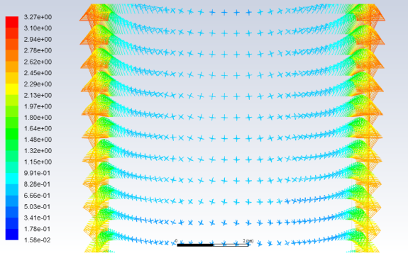
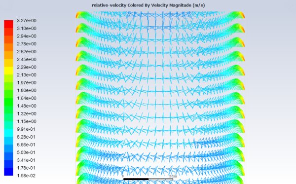
When you solve a problem in a moving reference frame, you can plot or report both absolute and relative velocities. For all velocity parameters (for example, Velocity Magnitude and Mach Number), corresponding relative values will be available for postprocessing (for example, Relative Velocity Magnitude and Relative Mach Number). These variables are contained in the Velocity... category of the variable selection drop-down list that appears in postprocessing dialog boxes. Relative values are also available for postprocessing of total pressure, total temperature, and any other parameters that include a dynamic contribution dependent on the reference frame (for example, Relative Total Pressure, Relative Total Temperature, Rothalpy).
When plotting velocity vectors, you can choose to plot vectors in the absolute frame (the default), or you can select Relative Velocity in the Vectors of drop-down list in the Vectors Dialog Box to plot vectors in the moving frame. If you plot relative velocity vectors, you might want to color the vectors by relative velocity magnitude (by choosing Relative Velocity Magnitude in the Color by list); by default they will be colored by absolute velocity magnitude. Figure 10.6: Absolute Velocity Vectors and Figure 10.7: Relative Velocity Vectors show absolute and relative velocity vectors in a moving domain with a stationary outer wall.