


This section describes the algorithms available in Ansys Fluent to model the fluctuating velocity at velocity inlet boundaries or pressure inlet boundaries.
The stochastic components of the flow at the velocity-specified inlet boundaries are neglected if the No Perturbations option is used. In such cases, individual instantaneous velocity components are simply set equal to their mean velocity counterparts. This option is suitable only when the level of turbulence at the inflow boundaries is negligible or does not play a major role in the accuracy of the overall solution.
Important: The methods listed below are available for velocity inlet and pressure inlet boundary conditions. For the velocity inlet, the fluctuations are added on the mean specified velocity. For the pressure inlet, virtual body forces are employed in the momentum equations to add the reconstructed turbulent fluctuations to the velocity field. These virtual body forces are considered only in the first cells close to the inlet.
The methods are available for the SAS, DES, SDES, SBES, and LES models. If unsteadiness inside the domain can be sustained depends on the flow and the grid spacing, especially when using the SAS or the DDES models for wall bounded flows.
These methods require realistic inlet conditions, such as providing U, k, and
 (or
(or  ) profiles, that can be obtained from separate RANS simulations. Unrealistic
("flat") turbulent profiles at inlets will generate unrealistic turbulent eddies at
inlets. Be aware of the order of the conversion operations applied to the inlet velocity and to
the turbulence quantities, which is explained in Estimating Turbulent Kinetic Energy from Turbulence Intensity. This conversion order is important when computing the fluctuation
amplitudes based on the specified turbulence intensity. It can also influence other properties
of the generated synthetic turbulence, for example the global time scale
) profiles, that can be obtained from separate RANS simulations. Unrealistic
("flat") turbulent profiles at inlets will generate unrealistic turbulent eddies at
inlets. Be aware of the order of the conversion operations applied to the inlet velocity and to
the turbulence quantities, which is explained in Estimating Turbulent Kinetic Energy from Turbulence Intensity. This conversion order is important when computing the fluctuation
amplitudes based on the specified turbulence intensity. It can also influence other properties
of the generated synthetic turbulence, for example the global time scale  of the Synthetic Turbulence Generator, see Equation 4–337. This time scale depends on the inlet velocity, which may
first be converted according to the Velocity Formulation selected in the General Task Page.
of the Synthetic Turbulence Generator, see Equation 4–337. This time scale depends on the inlet velocity, which may
first be converted according to the Velocity Formulation selected in the General Task Page.
To generate a time-dependent inlet condition, a random 2D vortex method is considered. With
this approach, a perturbation is added on a specified mean velocity profile via a fluctuating
vorticity field (that is, two-dimensional in the plane normal to the streamwise direction). The
vortex method is based on the Lagrangian form of the 2D evolution equation of the vorticity and
the Biot-Savart law. A particle discretization is used to solve this equation. These particles,
or "vortex points" are convected randomly and carry information about the vorticity
field. If  is the number of vortex points and
  is the area of the inlet section, the amount of vorticity carried by a given
particle
is the area of the inlet section, the amount of vorticity carried by a given
particle  is represented by the circulation
  and an assumed spatial distribution
  :
:
 | (4–330) |
 | (4–331) |
where  is the turbulence kinetic energy. The parameter
  provides control over the size of a vortex particle. The resulting
discretization for the velocity field is given by
provides control over the size of a vortex particle. The resulting
discretization for the velocity field is given by
 | (4–332) |
Where  is the unit vector in the streamwise direction. Originally [588], the size of the vortex was fixed by an ad hoc value of
  . To make the vortex method generally applicable, a local vortex size is
specified through a turbulent mixing length hypothesis.
. To make the vortex method generally applicable, a local vortex size is
specified through a turbulent mixing length hypothesis.  is calculated from a known profile of mean turbulence kinetic energy and mean
dissipation rate at the inlet according to the following:
is calculated from a known profile of mean turbulence kinetic energy and mean
dissipation rate at the inlet according to the following:
 | (4–333) |
where  . To ensure that the vortex will always belong to resolved scales, the minimum
value of
. To ensure that the vortex will always belong to resolved scales, the minimum
value of  in Equation 4–333 is bounded by the local grid size.
The sign of the circulation of each vortex is changed randomly each characteristic time scale
. In the general implementation of the vortex method, this time scale
represents the time necessary for a 2D vortex convected by the bulk velocity in the boundary
normal direction to travel along
in Equation 4–333 is bounded by the local grid size.
The sign of the circulation of each vortex is changed randomly each characteristic time scale
. In the general implementation of the vortex method, this time scale
represents the time necessary for a 2D vortex convected by the bulk velocity in the boundary
normal direction to travel along  times its mean characteristic 2D size (
 ), where
  is fixed equal to 100 from numerical testing. The vortex method considers only
velocity fluctuations in the plane normal to the streamwise direction.
is fixed equal to 100 from numerical testing. The vortex method considers only
velocity fluctuations in the plane normal to the streamwise direction.
In Ansys Fluent however, a simplified linear kinematic model (LKM) for the streamwise velocity
fluctuations is used [414]. It is derived from a linear model that
mimics the influence of the two-dimensional vortex in the streamwise mean velocity field. If the
mean streamwise velocity  is considered as a passive scalar, the fluctuation
  resulting from the transport of
  by the planar fluctuating velocity field
  is modeled by
 | (4–334) |
where  is the unit vector aligned with the mean velocity gradient
  . When this mean velocity gradient is equal to zero, a random perturbation can
be considered instead.
. When this mean velocity gradient is equal to zero, a random perturbation can
be considered instead.
Since the fluctuations are equally distributed among the velocity components, only the
prescribed kinetic energy profile can be fulfilled at the inlet of the domain. Farther
downstream, the correct fluctuation distribution is recovered [414].
However, if the distribution of the normal fluctuations is known or can be prescribed at the
inlet, a rescaling technique can be applied to the synthetic flow field in order to fulfill the
normal statistic fluctuations  ,
,  , and
, and  as given at the inlet.
With the rescaling procedure, the velocity fluctuations are expressed according to:
 | (4–335) |
This also results in an improved representation of the turbulent flow field downstream of the inlet. This rescaling procedure is used only if the Reynolds-Stress Components is specified as the Reynolds-Stress Specification Method, instead of the default option K or Turbulence Intensity.
Note: Mass conservation is not enforced for the velocity fluctuations generated by the Vortex Method. This can lead to unexpected pressure fluctuations and artificial disturbances or noise when solving acoustics. To remedy this problem, you can enable mass conservation for the vortex method by selecting Satisfy Mass Conservation? on the inlet dialog box.
Important: Since the vortex method theory is based on the modification of the velocity field normal
to the streamwise direction, it is imperative that you create an inlet plane normal (or as
close as possible) to the streamwise velocity direction. Problems can arise if the inlet
convective velocity is of the same order or lower than  , as this can cause local outflow. For this reason it should be applied with
caution for Tu~1 or smaller).
, as this can cause local outflow. For this reason it should be applied with
caution for Tu~1 or smaller).
The vortex method covers the entire boundary for which it is selected with vortices, even in regions, where the incoming turbulence level is low (freestream). For efficiency reasons, it is therefore recommended that you restrict the domain of the VM to the region where you which to generate unsteady turbulence. As an example, assume a thin mixing layer enters through a much larger inlet region. It is then advised to split the inlet boundary into three parts. One below the mixing layer with constant inlet velocity, one where the mixing layer enters the domain using the VM and a third above the mixing layer, again with a constant velocity. Thereby the vortices are concentrated at the domain of interest. Otherwise, a very large number of vortices would have to be generated to ensure a sufficient number of them in the thin mixing layer region.
The spectral synthesizer provides an alternative method of generating fluctuating velocity components. It is based on the random flow generation technique originally proposed by Kraichnan [322] and modified by Smirnov et al. [605]. In this method, fluctuating velocity components are computed by synthesizing a divergence-free velocity-vector field from the summation of Fourier harmonics. In Ansys Fluent, the default number of Fourier harmonics is set to 250.
To generate time-dependent inlet conditions for scale resolving turbulence simulations, a Fourier based synthetic turbulence generator is used.
This method is inexpensive in terms of computational time compared with the other existing methods while achieving high quality turbulence fluctuations.
The velocity vector at a point  of an inlet boundary condition is specified as the sum of the mean velocity
vector and the vector of synthetic velocity fluctuations:
of an inlet boundary condition is specified as the sum of the mean velocity
vector and the vector of synthetic velocity fluctuations:
 | (4–336) |
The field of velocity fluctuations  is defined as the superposition of weighted spatio-temporal Fourier modes
scaled such that the corresponding kinetic energy of the inflow is equal to the prescribed RANS
kinetic energy
is defined as the superposition of weighted spatio-temporal Fourier modes
scaled such that the corresponding kinetic energy of the inflow is equal to the prescribed RANS
kinetic energy  at the inlet boundary:
 | (4–337) |
where:
 is the number of modes.
 is the normalized amplitude of the mode
  defined by the local energy spectrum.
 is the amplitude of the wave number vector of the mode
  .
.
 is a random unit vector of direction uniformly distributed over a
sphere.
is a random unit vector of direction uniformly distributed over a
sphere.
 is a unit vector normal to
  (
( ), and in turn the angle defining its direction in the plane normal to
 is a random number uniformly distributed in the interval (0,2
 ).
).
 is the phase of the mode
  , which is also a random number uniformly distributed in the interval
(0,2
, which is also a random number uniformly distributed in the interval
(0,2 ).
).
 is the non-dimensional frequency of the mode
  with Gaussian distribution and the mean value and standard deviation equal to
2
with Gaussian distribution and the mean value and standard deviation equal to
2 .
.
 is the global time-scale. It is based on the characteristic length and
velocity scales defined as the maximum RANS turbulence length scale and velocity at the inlet
zone.
is the global time-scale. It is based on the characteristic length and
velocity scales defined as the maximum RANS turbulence length scale and velocity at the inlet
zone.
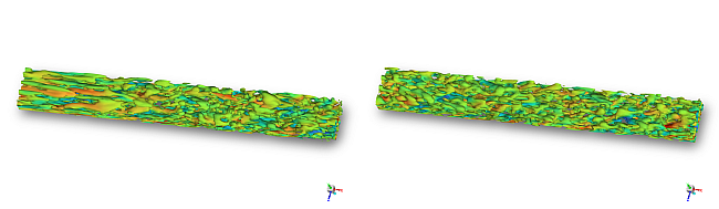
Important: Using the entire inlet zone to determine the characteristic scales may lead to incorrect
results if only a small section of the inlet face zone generates synthetic turbulence. For
example, unrealistically long turbulent structures can be generated in the turbulent boundary
layer if the RANS turbulent length scale in the free stream is arbitrarily high. In such
situations, it is necessary to limit the area of computation for the global scales to the
relevant part of the inlet only, the effect of which can be seen in the figure below. To limit
the search area, the Scale Search Limiters can be specified:
Turbulent Intensity, Turbulent
Viscosity Ratio, or Wall Distance Threshold.
Velocity and length scales are then computed using only the part of inlet face zone where the
corresponding inlet turbulent parameter is higher than the specified threshold values
(Turbulent Intensity, Turbulent
Viscosity Ratio) or simply where the distance to the wall is smaller than the
specified Wall Distance Threshold value. Limiters can be
specified on the Velocity or Pressure Inlet dialog boxes or using the console command to set
boundary conditions (/define/boundary-conditions/set).
Figure 4.11: Turbulent Structures Generated by Synthetic Turbulence Generator in the Boundary Layer with Arbitrarily High Turbulent Length Scale in the Free Stream: With Scale Search Limiter Option Set to None (left) and with Specified Turbulent Intensity Threshold 2% (right)
The face based (default) synthetic turbulence generator generates spurious pressure fluctuations making it unfit for aeroacoustics simulations. The volumetric version, available only for the omega-based SBES models, can be enabled for velocity or pressure inlets by selecting Volumetric Forcing?. It avoids generating undesirable noise by introducing volumetric sources of turbulent fluctuations into the momentum equations within a three dimensional forcing zone starting from the boundary. The reduction in noise allows the synthetic turbulence generator to be applied to acoustic tasks.
Inside the volumetric forcing region, the SBES model works in LES mode and that can cause inaccuracies in the presence of boundary layers (for example, if the volumetric synthetic turbulence generation is applied to a boundary condition that is connected to a wall). The SBES model behavior can be checked by visualizing the SBES blending function.
You have the option of specifying an Automatic (based on turbulence length scale) forcing zone thickness or directly setting the forcing zone thickness via a Specified Value.
Note: Unlike the Vortex Method, mass conservation for the Synthetic Turbulence Generator is enabled by default and cannot be disabled.
For further details, see [594].
A universal implementation of the volumetric forcing is a challenging task, since it requires a correct identification of the forcing zone. In the current version of this method in Ansys Fluent, all cells in a cell zone adjacent to the considered inlet zone are marked for the forcing, which are located within the forcing zone thickness counted from the inlet zone. The distance between each cell center and the inlet zone center is calculated along the normal-to-inlet direction. In the parallel-to-inlet direction the marked cell layer may be larger that the inlet zone. However, the forcing intensity is scaled with the modeled turbulence kinetic energy, which results from its transport equation. Therefore, outside of the turbulent stream coming from the adjacent inlet zone, the forcing intensity is zero. When, however, the marked cell layer crosses other turbulent parts of the solution field, this will generate forcing also in those parts, which is normally undesirable. Such situation is illustrated in Figure 4.12: Splitting of a cell zone in a complex flow simulation to avoid the undesirable side effect of the volumetric forcingFigure 4.12.
Figure 4.12: Splitting of a cell zone in a complex flow simulation to avoid the undesirable side effect of the volumetric forcing
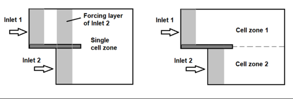
In such cases splitting a large cell zone in smaller parts helps to limit the marked cell layer and to avoid spurious forcing in undesired locations.