


The standard boundary conditions, when imposed on the boundaries of an artificially truncated domain, result in the reflection of the outgoing pressure waves. As a consequence, the interior domain will contain spurious wave reflections. Many applications require precise control of the wave reflections from the domain boundaries to obtain accurate flow solutions. Ansys Fluent offers several boundary wave models that can be used to at the domain boundaries to control these spurious wave reflections.
The following boundary acoustic wave models are available:
turbo-specific non-reflecting boundary condition (NRBC) (density-based solver only)
general NRBC (pressure-based and density-based solvers)
impedance boundary condition (pressure-based solver only)
transparent flow forcing (pressure-based solver only)
In the density-based solver, the NRBC models are available for flows using the compressible ideal-gas law.
In the pressure-based solver, the general NRBC, impedance, and transient flow forcing models available for transient simulations of compressible flows (including the ideal-gas law, real gas law, species transport, and compressible mixture models).
Information about the available boundary acoustic wave models is provided in the following sections.
Note: An alternative to the boundary acoustic wave models is to define sponge layers at boundary zones. Such sponge layers are based on the density, and are only available in a transient simulation for a compressible flow with the pressure-based solver. For details, see Sponge Layers.
Information about turbo-specific NRBCs is provided in the following sections.
The standard pressure boundary conditions for compressible flow fix specific flow variables at the boundary (for example, static pressure at an outlet boundary). As a result, pressure waves incident on the boundary will reflect in an unphysical manner, leading to local errors. The effects are more pronounced for internal flow problems where boundaries are usually close to geometry inside the domain, such as compressor or turbine blade rows.
The turbo-specific non-reflecting boundary conditions permit waves to “pass” through the boundaries without spurious reflections. The method used in Ansys Fluent is based on the Fourier transformation of solution variables at the non-reflecting boundary [52]. Similar implementations have been investigated by other authors [102] [135]. The solution is rearranged as a sum of terms corresponding to different frequencies, and their contributions are calculated independently. While the method was originally designed for axial turbomachinery, it has been extended for use with radial turbomachinery.
Note the following limitations of turbo-specific NRBCs:
They are available only with the density-based solver (explicit or implicit).
The current implementation applies to steady compressible flows, with the density calculated using the ideal gas law.
Inlet and outlet boundary conditions must be pressure inlets and outlets only.
Important: Note that the pressure inlet boundaries must be set to the cylindrical coordinate flow specification method when turbo-specific NRBCs are used.
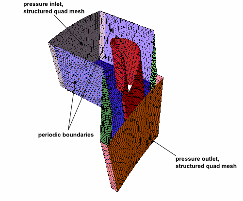
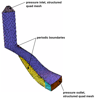
Quad-mapped (structured) surface meshes must be used for inflow and outflow boundaries in a 3D geometry (that is, triangular or quad-paved surface meshes are not allowed). See Figure 7.83: Mesh and Prescribed Boundary Conditions in a 3D Axial Flow Problem and Figure 7.84: Mesh and Prescribed Boundary Conditions in a 3D Radial Flow Problem for examples.
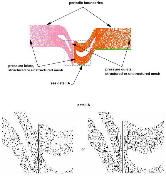
Important: Note that you may use unstructured meshes in 2D geometries (Figure 7.85: Mesh and Prescribed Boundary Conditions in a 2D Case), and an unstructured mesh may be used away from the inlet and outlet boundaries in 3D geometries.
The turbo-specific NRBC [52] has been extended for use on 3D geometries [135] by decoupling the tangential flow variations from the radial variations. This approximation works best for geometries with a blade pitch that is small compared to the radius of the geometry.
Reverse flow on the inflow and outflow boundaries are not allowed. If strong reverse flow is present, then you should consider using the General NRBCs instead.
NRBCs are not compatible with species transport models. They are mainly used to solve ideal-gas single-species flow.
Turbo-specific NRBCs are based on Fourier decomposition of solutions to the linearized Euler equations. The solution at the inlet and outlet boundaries is circumferentially decomposed into Fourier modes, with the 0th mode representing the average boundary value (which is to be imposed as a user input), and higher harmonics that are modified to eliminate reflections [135].
In order to treat individual waves, the linearized Euler equations are transformed to characteristic variable
( ) form. If we first consider the 1D form of the linearized Euler equations, it can be shown that the
characteristic variables
) form. If we first consider the 1D form of the linearized Euler equations, it can be shown that the
characteristic variables  are related to the solution variables as follows:
 | (7–153) |
where
 | (7–154) |
where  is the average acoustic speed along a boundary zone,
  ,
,  ,
,  ,
,  , and
, and  represent perturbations from a uniform condition (for example,
  , and so on).
Note that the analysis is performed using the cylindrical coordinate system. All overlined (averaged) flow field variables
(for example,  ,
,  ) are intended to be averaged along the pitchwise direction.
In quasi-3D approaches [52] [102] [135], a
procedure is developed to determine the changes in the characteristic variables, denoted by  , at the boundaries such that waves will not reflect. These changes in characteristic variables are
determined as follows:
, at the boundaries such that waves will not reflect. These changes in characteristic variables are
determined as follows:
 | (7–155) |
where
 | (7–156) |
The changes to the outgoing characteristics — one characteristic for subsonic inflow ( ), and four characteristics for subsonic outflow (
 ,
,  ,
,  ,
,  ) — are determined from extrapolation of the flow field variables using Equation 7–155.
The changes in the incoming characteristics — four characteristics for subsonic inflow ( ,
,  ,
,  ,
,  ), and one characteristic for subsonic outflow (
 ) — are split into two components: average change along the boundary (
 ), and local changes in the characteristic variable due to harmonic variation along the boundary
(
), and local changes in the characteristic variable due to harmonic variation along the boundary
( ). The incoming characteristics are therefore given by
 | (7–157) |
 | (7–158) |
where  on the inlet boundary or
  on the outlet boundary, and
  is the grid index in the pitchwise direction including the periodic point once. The under-relaxation factor
 has a default value of
  . Note that this method assumes a periodic solution in the pitchwise direction.
The flow is decomposed into mean and circumferential components using Fourier decomposition. The 0th Fourier mode corresponds to the average circumferential solution, and is treated according to the standard 1D characteristic theory. The remaining parts of the solution are described by a sum of harmonics, and treated as 2D non-reflecting boundary conditions [52].
For subsonic inflow, there is one outgoing characteristic ( ) determined from Equation 7–155, and four incoming characteristics (
 ,
,  ,
,  ,
,  ) calculated using Equation 7–157. The average changes in the incoming characteristics
are computed from the requirement that the entropy (
) calculated using Equation 7–157. The average changes in the incoming characteristics
are computed from the requirement that the entropy ( ), radial and tangential flow angles (
 and
and  ), and stagnation enthalpy (
 ) are specified. Note that in Ansys Fluent you can specify
  and
and  at the inlet, from which
  and
and  are easily obtained. This is equivalent to forcing the following four residuals to be zero:
 | (7–159) |
 | (7–160) |
 | (7–161) |
 | (7–162) |
where
 | (7–163) |
 | (7–164) |
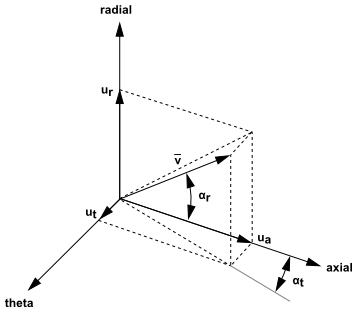
The average characteristic is then obtained from residual linearization as follows (see also Figure 7.86: Prescribed Inlet Angles
 | (7–165) |
where
 | (7–166) |
 | (7–167) |
 | (7–168) |
and
 | (7–169) |
 | (7–170) |
 | (7–171) |
where
 | (7–172) |
 | (7–173) |
 | (7–174) |
 | (7–175) |
 | (7–176) |
 | (7–177) |
To address the local characteristic changes at each  grid point along the inflow boundary, the following relations are developed [52] [135]:
 | (7–178) |
Note that the relation for the first and fourth local characteristics force the local entropy and stagnation enthalpy to match their average steady-state values.
The characteristic variable  is computed from the inverse discrete Fourier transform of the second characteristic. The discrete Fourier
transform of the second characteristic in turn is related to the discrete Fourier transform of the fifth characteristic.
Hence, the characteristic variable
is computed from the inverse discrete Fourier transform of the second characteristic. The discrete Fourier
transform of the second characteristic in turn is related to the discrete Fourier transform of the fifth characteristic.
Hence, the characteristic variable  is computed along the pitch as follows:
 | (7–179) |
The Fourier coefficients  are related to a set of equidistant distributed characteristic variables
  by the following [102]:
 | (7–180) |
where
 | (7–181) |
and
 | (7–182) |
The set of equidistributed characteristic variables  is computed from arbitrary distributed
  by using a cubic spline for interpolation, where
 | (7–183) |
For supersonic inflow the user-prescribed static pressure ( ) along with total pressure (
 ) and total temperature (
 ) are sufficient for determining the flow condition at the inlet.
For subsonic outflow, there are four outgoing characteristics ( ,
,  ,
,  , and
, and  ) calculated using Equation 7–155, and one incoming characteristic (
 ) determined from Equation 7–157. The average change in the incoming fifth
characteristic is given by
) determined from Equation 7–157. The average change in the incoming fifth
characteristic is given by
 | (7–184) |
where  is the current averaged pressure at the exit plane and
  is the desirable average exit pressure (this value is specified by you for single-blade calculations or
obtained from the assigned profile for mixing-plane calculations). The local changes (
is the desirable average exit pressure (this value is specified by you for single-blade calculations or
obtained from the assigned profile for mixing-plane calculations). The local changes ( ) are given by
 | (7–185) |
The characteristic variable  is computed along the pitch as follows:
 | (7–186) |
The Fourier coefficients  are related to two sets of equidistantly distributed characteristic variables (
 and
and  , respectively) and given by the following [102]:
 | (7–187) |
where
 | (7–188) |
 | (7–189) |
The two sets of equidistributed characteristic variables ( and
and  ) are computed from arbitrarily distributed
  and
and  characteristics by using a cubic spline for interpolation, where
 | (7–190) |
 | (7–191) |
For supersonic outflow all flow field variables are extrapolated from the interior.
Once the changes in the characteristics are determined on the inflow or outflow boundaries, the changes in the flow
variables  can be obtained from Equation 7–155. Therefore, the values of the flow variables at
the boundary faces are as follows:
can be obtained from Equation 7–155. Therefore, the values of the flow variables at
the boundary faces are as follows:
 | (7–192) |
 | (7–193) |
 | (7–194) |
 | (7–195) |
 | (7–196) |
Important: If you intend to use turbo-specific NRBCs in conjunction with the density-based implicit solver, it is recommended that you first converge the solution before turning on turbo-specific NRBCs, then converge it again with turbo-specific NRBCs turned on. If the solution is diverging, then you should lower the CFL number. These steps are necessary because only approximate flux Jacobians are used for the pressure-inlet and pressure-outlet boundaries when turbo-specific NRBCs are activated with the density-based implicit solver.
The procedure for using the turbo-specific NRBCs is as follows:
Turn on the turbo-specific NRBCs using the
non-reflecting-bctext command:define→boundary-conditions→non-reflecting-bc→turbo-specific-nrbc→enable?If you are not sure whether or not NRBCs are turned on, use the
show-statustext command.Perform NRBC initialization using the
initializetext command:define→boundary-conditions→non-reflecting-bc→turbo-specific-nrbc→initializeIf the initialization is successful, a summary printout of the domain extent will be displayed. If the initialization is not successful, an error message will be displayed indicating the source of the problem. The initialization will set up the pressure-inlet and pressure-outlet boundaries for use with turbo-specific NRBCs.
Important: Note that the pressure inlet boundaries must be set to the cylindrical coordinate flow specification method when turbo-specific NRBCs are used.
If necessary, modify the parameters in the
set/submenu:define→boundary-conditions→non-reflecting-bc→turbo-specific-nrbc→set-
under-relaxation allows you to set the value of the under-relaxation factor
 in Equation 7–157. The default value is
  .
.-
discretization allows you to set the discretization scheme. The default is to use higher-order reconstruction if available.
-
verbosity allows you to control the amount of information printed to the console during an NRBC calculation.
0: silent1: basic information (default)2: detailed information (for debugging purposes only)
-
If you want to use the NRBCs with the mixing-plane model you must define the mixing plane interfaces as pressure-outlet and pressure-inlet zone type pairs.
Important: Turbo-specific NRBCs should not be used with the mixing-plane model if reverse flow is present across the mixing-plane.
When the turbo-specific NRBCs are used in conjunction with the parallel solver, all cells in each boundary zone, where NRBCs will be applied, must be located or contained within a single partition. You can ensure this by manually partitioning the mesh (see Partitioning the Mesh Manually and Balancing the Load for more information).
Information about general NRBCs is provided in the following sections.
The general non-reflecting boundary conditions in Ansys Fluent are based on characteristic wave relations derived from the
Euler equations. In the density-based solver, the non-reflecting boundary conditions are applied only on pressure-outlet boundary
conditions. In the pressure-based solver they are applied on pressure-inlet, pressure-outlet, velocity-inlet and mass-flux
boundary conditions. To obtain the primitive flow quantities ( ), reformulated Euler equations are solved on the boundary of the domain in an algorithm similar to the flow
equations applied to the interior of the domain.
), reformulated Euler equations are solved on the boundary of the domain in an algorithm similar to the flow
equations applied to the interior of the domain.
Unlike the turbo-specific NRBC, the general NRBC method is not restricted by geometric constraints or mesh type. However, good cell skewness near the boundaries where the NRBCs can be applied for better convergence.
Note the following restrictions and limitations on the general NRBCs:
The general NRBC is not available if the target mass flow rate is activated in the pressure-outlet dialog box.
The general NRBC using the density-based solver is available only with compressible flow while using the ideal-gas law.
Important: The general NRBC using the density-based solver should not be used with the wet steam or real gas models.
The general NRBCs using the density-based solver are not compatible with species transport and mixture fraction transport models (for premixed and partially-premixed models). They are mainly used to solve ideal-gas single-component flow.
The general NRBCs using the pressure-based solver are not compatible with steady-state cases or the Eulerian multiphase model. For VOF or mixture multiphase cases that involve compressible gases or compressible liquids, only pressure inlets and pressure outlets can enable the non-reflecting boundary condition option. Note that some small reflections may still occur from NRBC boundaries when secondary-phase volume fractions are nonzero at the boundaries.
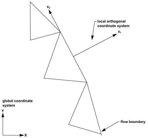
General NRBCs are derived by first recasting the Euler equations in an orthogonal coordinate system ( ) such that one of the coordinates,
  , is normal to the boundary Figure 7.87: The Local Orthogonal Coordinate System onto which Euler Equations are Recasted for the General NRBC Method. The characteristic analysis [163] [164] is then used to modify terms corresponding to waves propagating
in the
, is normal to the boundary Figure 7.87: The Local Orthogonal Coordinate System onto which Euler Equations are Recasted for the General NRBC Method. The characteristic analysis [163] [164] is then used to modify terms corresponding to waves propagating
in the  normal direction. When doing so, a system of equations can be written to describe the wave propagation as
follows:
normal direction. When doing so, a system of equations can be written to describe the wave propagation as
follows:
 | (7–197) |
Where  ,
,  and
and  and
and  ,
,  and
and  are the velocity components in the coordinate system (
 ,
,  ,
,  ). The equations above are solved on non-reflecting boundaries, along with the interior governing flow
equations, using similar time stepping algorithms to obtain the values of the primitive flow variables (
). The equations above are solved on non-reflecting boundaries, along with the interior governing flow
equations, using similar time stepping algorithms to obtain the values of the primitive flow variables ( ).
).
Important: Note that a transformation between the local orthogonal coordinate system ( ,
,  ,
,  ) and the global Cartesian system (X, Y, Z) must be defined on each face on the boundary to obtain the
velocity components (
) and the global Cartesian system (X, Y, Z) must be defined on each face on the boundary to obtain the
velocity components ( ,
,  ,
,  ) in a global Cartesian system.
Figure 7.87: The Local Orthogonal Coordinate System onto which Euler Equations are Recasted for the General NRBC Method
The  terms in the transformed Euler equations contain the outgoing and incoming characteristic wave amplitudes,
 , and are defined as follows:
 | (7–198) |
From characteristic analyses, the wave amplitudes,  , are given by:
 | (7–199) |
The outgoing and incoming characteristic waves are associated with the characteristic velocities of the system (i.e
eigenvalues),  , as seen in Figure 7.88: Waves Leaving and Entering a Boundary Face on Inflow and Outflow Boundaries. The Wave Amplitudes are Shown with the
Associated Eigenvalues for a Subsonic Flow Condition. These eigenvalues are given by:
, as seen in Figure 7.88: Waves Leaving and Entering a Boundary Face on Inflow and Outflow Boundaries. The Wave Amplitudes are Shown with the
Associated Eigenvalues for a Subsonic Flow Condition. These eigenvalues are given by:
 | (7–200) |
Figure 7.88: Waves Leaving and Entering a Boundary Face on Inflow and Outflow Boundaries. The Wave Amplitudes are Shown with the Associated Eigenvalues for a Subsonic Flow Condition
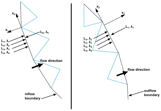
For subsonic flow leaving a boundary, four waves leave the domain (associated with positive eigenvalues  ,
,  ,
,  , and
, and  ) and one enters the domain (associated with negative eigenvalue
  ). For subsonic flow entering a boundary, four waves enter the domain (associated with the negative eigenvalues
 ,
,  ,
,  ,
,  ) and one leaves the domain (associated with a positive eigenvalue
  ).
).
To solve Equation 7–197 on a boundary, the amplitude of the incoming and outgoing waves must be
first determined. The amplitude of outgoing waves are computed from Equation 7–199 by using
extrapolated values of flow derivatives  ,
,  ,
,  ,
,  , and
, and  from inside the domain. The amplitude of the incoming waves are computed as follows. The amplitude of waves
 ,
,  , for tangential velocity components, is set to zero. The amplitude of the incoming pressure and entropy waves
are computed from the Linear Relaxation Method (LRM) of Poinsot [120] [121]. The LRM method sets the value of the incoming wave amplitude to be proportional to the differences between the local primitive
variable on a boundary face and the imposed boundary value. The expression for the amplitudes depends on the boundary type as
shown below:
, for tangential velocity components, is set to zero. The amplitude of the incoming pressure and entropy waves
are computed from the Linear Relaxation Method (LRM) of Poinsot [120] [121]. The LRM method sets the value of the incoming wave amplitude to be proportional to the differences between the local primitive
variable on a boundary face and the imposed boundary value. The expression for the amplitudes depends on the boundary type as
shown below:
Pressure Outlet

(7–201)
where
 is the imposed pressure at the exit boundary,
  is the relaxation factor, and
  is the local pressure value at the boundary.
In general, the desirable average pressure on a non-reflecting boundary can be either relaxed toward a pressure value at infinity or enforced to be equivalent to some desired pressure at the exit of the boundary.
In the case of a backflow, the pressure-based solver has two options for specifying pressure at the boundary; static pressure or total pressure. If the static pressure option is selected, the pressure at infinity is equal to the pressure defined in the boundary dialog box. If the total pressure option is selected, the pressure at infinity is a total pressure that is computed from the value in the dialog box. For the density-based solver, the total pressure option is used and no other options are available.
If you want the average pressure at the boundary to relax toward
 at infinity (that is
  ), the suggested
  factor is given by:
(7–202)
where
 is the acoustic speed,
  is the domain size,
  is the maximum Mach number in the domain, and
  is the under-relaxation factor (default value is 0.15). On the other hand, if the desired average
pressure at the boundary is to approach a specific imposed value at the boundary, then the
is the under-relaxation factor (default value is 0.15). On the other hand, if the desired average
pressure at the boundary is to approach a specific imposed value at the boundary, then the  factor is given by:
(7–203)
where the default value for
 is 5.0
Important: The desired average pressure option is only available for the density-based solver.
Pressure Inlet:

(7–204)
where the imposed pressure,
 , and density,
  , are computed from the specified total pressure and total temperature.
Mass Flux Boundary:

(7–205)
where the imposed exit velocity and density are computed from specific mass flux and total temperature.
Velocity Inlet:

(7–206)
where the imposed velocity,
 , is specified at the boundary and the imposed density is computed from the specified boundary
temperature and extrapolated pressure.
, is specified at the boundary and the imposed density is computed from the specified boundary
temperature and extrapolated pressure.
The general Non-Reflecting Boundary Condition is available for use in the Pressure Outlet dialog box when either the density-based (with ideal gas law) or pressure-based solvers are activated to solve for compressible flows. The general Non-Reflecting Boundary Condition is available for use in the Pressure Inlet, Mass-Flow Inlet, and Velocity Inlet dialog boxes when the pressure-based solver is activated to solve for compressible flows.
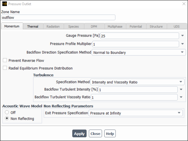
The example below shows you how to enable the general Non-Reflecting Boundary Condition in the Pressure Outlet dialog box. You would follow similar steps for the other boundary condition types mentioned above.
Select pressure-outlet from the Boundary Conditions task page and click the button.
In the Pressure Outlet dialog box, choose Non Reflecting under Acoustic Wave Model.
For the density-based solver, select one of the two Exit Pressure Specification options: Pressure at Infinity or Average Boundary Pressure. The pressure-based solver uses the Pressure at Infinity option and the Exit Pressure Specification drop-down list is not available.
The Pressure at Infinity boundary is typically used in unsteady calculations or when the exit pressure value is imposed at infinity. The boundary is designed so that the pressure at the boundary relaxes toward the imposed pressure at infinity. The speed at which this relaxation takes place is controlled by the parameter,
sigma, which can be adjusted in the TUI:define→boundary-conditions→non-reflecting-bc→general-nrbc→setIn the
set/submenu, you can set thesigmavalue. The default value forsigmais 0.15.The Average Boundary Pressure specification is usually used in steady-state calculations when you want to force the average pressure on the boundary to approach the exit pressure value. The matching of average exit pressure to the imposed average pressure is controlled by the parameter
sigma2which can be adjusted in the TUI:define→boundary-conditions→non-reflecting-bc→general-nrbc→setIn the
set/submenu, you can set thesigma2value. The default value forsigma2is 5.0.
Important: There is no guarantee that the
sigma2value of 5.0 will force the average boundary pressure to match the specified exit pressure in all flow situations. In the case where the desired average boundary pressure has not been achieved, you can intervene to adjust thesigma2value so that the desired average pressure on the boundary is approached.For the pressure-based solver, you can select one of two Backflow Pressure Specification options: Static Pressure or Total Pressure. For the density-based solver, the Backflow Pressure Specification is not shown and the Total Pressure option is used by default. Note that backflow is not allowed for pressure inlets, mass-flow inlets, or velocity inlets.
Important: For the pressure-based solver, you should choose Direction Vector or From Neighboring Cell as the Backflow Direction Specification Method if the flow is tangential to the boundary. You should not select the Normal to the Boundary option for Backflow Direction Specification Method in this case because the face velocity components for this case will be computed from flux as zero during initialization. This initialization will cause the solver convergence to fail.
Usually, the solver can operate at higher CFL values without the NRBCs being turned on. Therefore, the best practice is to first achieve a good stable solution (not necessarily converged) before activating the non-reflecting boundary condition. In many flow situations, the CFL value must be reduced from the normal operation to keep the solution stable. This is particularly true with the density-based implicit solver since the boundary update is done in an explicit manner. A typical CFL value in the density-based implicit solver, with the NRBC activated, is 2.0 and 4.0 in the pressure-based solver.
The impedance boundary condition (IBC) lies in between a traditional reflective boundary condition and a fully non-reflective boundary condition. It provides the ability to specify a partial reflection in the range from full-reflection to no-reflection. Impedance is a complex value; it is the reflection that changes the amplitude and the phase of the incoming wave. The use of impedance boundary conditions comes in cases where the flow in the simulation is highly influenced by reflected waves from objects outside the computational domain. In such cases the acoustic wave interaction from the larger domain can be modeled in the smaller domain through the use of impedance boundary conditions.
The impedance boundary condition is available only in the pressure-based solver. It is incompatible with steady-state flow, multiphase, or compressible liquid models (compressible-liquid method for density).
Impedance specifies an acoustic resistance in the frequency domain. It is a characteristic of the properties of the media and specific geometry described by a ratio of the pressure perturbation to the normal velocity perturbation at the boundary (Blackstock [19]). The specific impedance is calculated as follows:
 | (7–207) |
where apostrophe denotes acoustic perturbation and hat denotes quantity in the frequency domain.
Fluent is a time domain solver. It cannot use the impedance from the frequency domain directly. The above expression and all its variables have to be converted to the time domain. After the conversion the relation between pressure and normal velocity perturbations is expressed through a convolution integral.
 | (7–208) |
If impedance,  , is unbounded in the time domain, then admittance is used (admittance is the inverse of impedance). Fluent
uses the reflection coefficient instead of impedance/admittance, to uniformly treat unbounded cases (Fung [47]). The reflection coefficient is a ratio between reflected and incoming wave amplitudes at the boundary. It is expressed
through the impedance as:
, is unbounded in the time domain, then admittance is used (admittance is the inverse of impedance). Fluent
uses the reflection coefficient instead of impedance/admittance, to uniformly treat unbounded cases (Fung [47]). The reflection coefficient is a ratio between reflected and incoming wave amplitudes at the boundary. It is expressed
through the impedance as:
 | (7–209) |
Using a reflection coefficient, the relation between pressure and normal velocity perturbation is:
 | (7–210) |
The discretized form of this expression is used in Fluent to connect acoustic pressure and normal velocity. The computed acoustic perturbations are superimposed onto the pressure and velocity from non-reflecting boundary condition equations. The non-reflecting boundary condition equations provide mean flow values at the boundary, which drive the flow in the domain.
The data for the reflection coefficient are available in the frequency domain. As such they usually do not satisfy the causality
and reality conditions. Fluent asks you to provide the reflection coefficient data in the form of a special approximation. This
approximation is based on the system theory, which ensures that the reflection coefficient in the time domain will satisfy the
above conditions (Fung [46]). The reflection coefficient is represented as a sum of zero, first and
second order systems. The zero system is described with a real value, the first order system is described with a real pole, and
the second order system is described with a pair of complex conjugate poles. Introducing a system variable,  the complete approximation for the reflection coefficient is:
 | (7–211) |
where  is a real term,
  is a number of real poles,
  and
and  are real pole and its amplitude,
  is a number of complex conjugate pole pairs,
  ,
,  are real and imaginary part of the complex conjugate pole,
  and
and  are real and imaginary part of the amplitude of the complex pole.
To obey the causality and reality conditions, real pole  , real
  and imaginary part
  of the complex conjugate pole should be positive. The passivity condition requires that the absolute value of
zero order term
of the complex conjugate pole should be positive. The passivity condition requires that the absolute value of
zero order term  be less than 1. The above restrictions are enforced in the user interface. In addition you should ensure that
the absolute value of the reflection coefficient computed by this formula is less than 1.
be less than 1. The above restrictions are enforced in the user interface. In addition you should ensure that
the absolute value of the reflection coefficient computed by this formula is less than 1.
The experimental data can be specific impedance, reflection coefficient, or absorption coefficient data, and can be obtained from measurements or from an acoustic solver. Processing these data using Fluent or a mathematics package will provide an approximation in terms of first and second order poles.
The example below shows you how to enable the impedance boundary condition (IBC) in the Pressure Outlet dialog box. Similarly, you can enable IBC in the Pressure Inlet, Velocity Inlet, and Mass-Flow Inlet dialog boxes for compressible flows with the pressure-based solver.
Select pressure-outlet from the Boundary Condition task page and click the button.
In the Pressure Outlet dialog box, choose Impedance under Acoustic Wave Model.
The dialog box will expand to reveal Impedance Parameters.
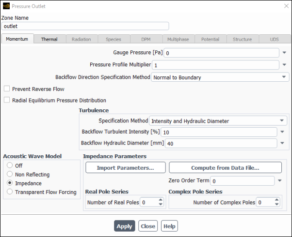
Specify the data for the reflection coefficient in the Impedance Parameters group box. This can be done using one of the following methods:
If you have a pole / residue file that contains the terms of the approximation formula (Equation 7–211), click the button and select the file; the values will then be automatically entered in the various fields of the Impedance Parameters group box. For information about the proper format of this file as well as how to generate one from experimental impedance data in the frequency domain, see Calculating Impedance Parameters.
If you have a data file that contains experimental impedance data in the frequency domain, click the button and use the Impedance Data Fitting dialog box that opens to compute the terms in the time domain and apply them to the various fields of the Impedance Parameters group box. For details, see Calculating Impedance Parameters.
Manually enter values in the various fields for the terms of the approximation formula (Equation 7–211):
Specify the Zero Order Term,
 .
.Under Real Pole Series, set the Number of Real Poles and for each real pole specify the Pole,
 , and the Amplitude,
  .
.Under Complex Pole Series, set the Number of Complex Poles and for each complex pole pair, specify Pole Real,
 , Pole Imaginary,
  , Amplitude Real,
  , and Amplitude Imaginary,
  .
.
Important: If flow is tangential to the boundary, then specify either From Neighboring Cell or Direction Vector for Back flow Direction Specification Method. Do not select Normal to the boundary because this computes the face velocity components from flux to zero values during initialization, which impairs solver convergence.
The IBC is implemented on top of the non-reflective boundary condition.
Note:
The mean flow in the domain should be well established before enabling IBC.
The cell acoustic Courant (CFL) number should be less than 1 in cells adjacent to the boundary where you define an impedance acoustic boundary condition. (For the definition of the Cell Acoustic Courant Number, refer to Field Function Definitions).
With the impedance acoustic boundary condition, you need to tighten the convergence criteria for continuity to 1e-4 in order to increase the number of coupling iterations between the impedance boundary condition calculation and the solver at each time step.
You can use Fluent to read experimental impedance data in the frequency domain and then compute the terms needed for an approximation of the reflection coefficient as a series of poles / residues in the time domain. The calculation uses an algorithm based on the work of Gustavsen and Semlyen [58]. The terms of the pole / residue series can be directly applied to the various fields of the Impedance Parameters group box of a boundary condition dialog box, saved as a pole / residue file (which can be useful for setting up multiple boundary conditions and/or case files), and/or printed in the console; you can also write the fitted frequency / impedance data to an output file, which you can compare to the input data to evaluate how well it fits.
Note: If you read experimental absorption coefficient data in the frequency domain, the terms of the pole / residue series that Fluent calculates may be different depending on which release or operating system you are using. Such differences will not affect the solution results, as only the curves of the fitted frequency / impedance data are used in the impedance boundary condition, and those curves will be consistent. You can verify this by comparing the output files of the fitted frequency / impedance data (see the steps that follow for details about writing such files).
To calculate and enter the impedance parameters, perform the following steps:
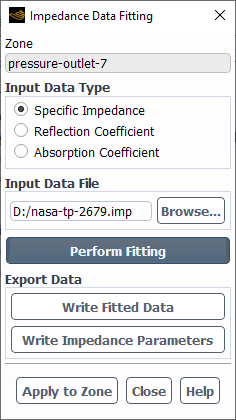
In the boundary condition dialog box (for example, the Pressure Outlet dialog box), click the button in the Impedance Parameters group box, to open the Impedance Data Fitting dialog box.
In the Impedance Data Fitting dialog box, make a selection from the Input Data Type for the experimental data in the frequency domain. The following types are available:
Specific Impedance
This corresponds to Equation 7–207.
Reflection Coefficient
This corresponds to Equation 7–209.
Absorption Coefficient
The absorption coefficient (
 ) is the ratio of the absorbed energy (
 ) to the incident energy (
 ):
):
(7–212)
It relates to the reflection coefficient as follows:

(7–213)
Enter the name of the Input Data File or use the button to select it. The file must be in monitor format, with separate columns for the frequency and the data values. The following are examples:
For a specific impedance data file named
nasa-tp-2679.imp:"nasa-tp-2679" "frequency" "impedance" ("frequency" "real" "imag") 5000. 0.41 -1.56 10000. 0.46 0.03 15000. 1.08 1.38 20000. 4.99 0.25 25000. 1.26 -1.53 30000. 0.69 -0.24For a reflection coefficient data file named
dc-real-complex-rf.rfl:"dc real complex fitting" "frequency" "reflection coefficient" ("frequency" "real" "imag") 150.0 0.6946227848755014 -0.08340940421826964 300.0 0.5785212268551001 -0.33760951170464315 450.0 0.3844647950039666 -0.36051768580559684 600.0 0.27881191269389494 -0.31875086372470873 750.0 0.22098593107397013 -0.2755872628668373 900.0 0.18674039023283218 -0.23974412499762482 1050.0 0.1650100694074955 -0.21097174097349292 1200.0 0.15043702854946334 -0.18781299172681953 1350.0 0.14022123873194448 -0.16894702736963293 1500.0 0.13279779044634915 -0.15336205026505353 1650.0 0.12724127578751093 -0.14031150077210966 1800.0 0.12297792604119287 -0.12924601721152512 1950.0 0.11963748299365515 -0.11975769596066593 2100.0 0.11697273089207115 -0.11153969759534471 2250.0 0.11481369319289189 -0.10435793597654594 2400.0 0.1130404841694425 -0.09803133050780145 2550.0 0.11156663966112866 -0.09241794300169018 2700.0 0.1103285600257371 -0.08740513783535145 2850.0 0.1092786384820483 -0.0829025079355948 3000.0 0.10838067800958853 -0.07883672147250274For an absorption coefficient data file named
dc-real-complex-ab.abs:"dc-real-complex-rf.in fitting" "frequency" "absorption coefficient" ("frequency" "value") 150.0 0.5105420580197505 300.0 0.5513330076846182 450.0 0.722213819623932 600.0 0.8206618042147218 750.0 0.8752168788129335 900.0 0.9076507811848114 1050.0 0.9282626015047457 1200.0 0.9420949805798284 1350.0 0.9517949061514425 1500.0 0.9588448283910658 1650.0 0.9641223404870439 1800.0 0.9681718967415641 1950.0 0.9713449669211347 2100.0 0.9738762760879893 2250.0 0.9759272370541228 2400.0 0.9776117071776074 2550.0 0.9790118087260594 2700.0 0.9801879507226298 2850.0 0.9811853533494976 3000.0 0.9820383999816481
Click the button to calculate the terms needed for an approximation of the reflection coefficient as a series of poles / residues in the time domain. The results are printed in the console (under
Zero Order Term,Number of Real Poles, and so on, which correspond to the terms for the reflection coefficient according to the approximation formula Equation 7–211).Note that prior to clicking the button, you have the option of revising a few additional settings for the fitting through the following text commands:
By default the algorithm will run 20 internal iterations; if this is inappropriate for your case, you can revise it using the following text command:
define/boundary-conditions/impedance-data-fitting/iterations.By default a convergence tolerance of 1e-6 is used for completing the iterative fitting procedure; if this is inappropriate for your case, you can revise it using the following text command:
define/boundary-conditions/impedance-data-fitting/convergence-tolerance.By default the minimum value of residues that are kept in the fitting is 1e-6. This residue check helps to eliminate parasitic poles. If the default value is inappropriate for your case, you can revise it using the following text command:
define/boundary-conditions/impedance-data-fitting/residue-tolerance.You can specify that messages are printed in the console as the fitting calculation progresses by entering the following text command:
define/boundary-conditions/impedance-data-fitting/verbosity
                                    1
.
(optional) Click the button to write a file with fitted frequency / impedance data. The number of lines corresponds to the number of lines in the input data file, and there are separate columns for the frequency and the real and imaginary values. This file can be compared to the input data to evaluate how well it fits.
(optional) Click the button to write a pole / residue file with the impedance parameters, which can then be imported using the button of a boundary condition dialog box. Such a file can be useful when setting up multiple boundary conditions and/or case files. The following is an example of the format of a pole / residue file:
Impedance parameters for nasa-tp-2679.imp:
Zero Order Term
6.227176322918e-01
Number of Real Poles
 0
Number of Complex Conjugate Poles
 2
Pole Real           Pole Imaginary      Amplitude Real       Amplitude Imaginary
3.462578756313e+03  5.077495917952e+03  -5.463369722031e+03  -2.849664452670e+03
4.754179871958e+03  1.663686613863e+04  -1.614972036282e+03  -5.411609140947e+03
Click the button to enter the results in the appropriate fields in the Impedance Parameters group box of the boundary condition dialog box.
Close the Impedance Data Fitting dialog box.
In the boundary condition dialog box, verify that the Impedance Parameters are appropriate and click the button.
As an alternative to using the Impedance Data Fitting dialog box in a Fluent session, you can instead use
the impedance utility to calculate the terms of the pole / residue series from a data file, print them,
and optionally write them to a file. This utility has some additional functionality, which may be useful in some circumstances. To
use the impedance utility, enter the following at a command prompt in a terminal or command window:
utility impedance [--help] [-p
P] [-f F] [-i I]
[-t T] [-r R]
[-y Y] [-m M]
[-v V] I [R C]
Note: The items enclosed in square brackets are optional. Do not type the square brackets.
--help(optional) prints the arguments available for theimpedanceutility.-pP (optional) specifies that the pole / residue mapping data is also written to an output file named P.-fF (optional) specifies that fitted frequency / impedance data is also written to an output file named F, with separate columns for the frequency and the real and imaginary values. This output file can be compared to the input data to evaluate how well it fits.-iI (optional) specifies that the algorithm uses a specified number (I) of internal iterations. By default, 20 iterations will be run.-tT (optional) sets the convergence tolerance (which is an accuracy that is used for completing the iterative fitting procedure) to T. By default, the tolerance is set to 1e-6.-rR (optional) sets the residue tolerance (that is, the minimum value of residues that are kept in the fitting) to R. This residue check helps to eliminate parasitic poles. By default, the residue tolerance is set to 1e-6.-yY (optional) specifies the type of data file you are reading. Y can beimpedance(for specific impedance data, which is the default),reflection(for reflection coefficient data), orabsorption(for absorption coefficient data).-mM (optional) can be used with-y absorption, and specifies the phase of the absorption coefficient. M can bezero(the default) orrandom.-vV (optional) sets the verbosity of the progress messages. V can be0(the default, which prints no progress messages during the calculation) or1(which prints messages in the console as the fitting calculation progresses).I must be replaced with the name of the input file, which provides experimental data in monitor format with separate columns for the frequency and the data.
R and C (optional) allow you to specify the number of poles (real and complex conjugate, respectively) that you want used during fitting. With this option, you must ensure that the numbers you enter are appropriate for the data you provide, such that:

(7–214)
where n is the number of data points in your input file. When multiple combinations of values for R and C can satisfy the previous equation, you should ensure that the values you use yield the lowest possible RMS error (which is the root mean square difference between the fit and the input data, and is printed at the end of the calculation).
Note: It is recommended that you omit R and C; when omitted, Fluent will automatically use numbers of poles that yield the lowest RMS error.
The following example demonstrates the use of the impedance utility from a command prompt, using the
input file described previously.
utility impedance nasa-tp-2679.imp -p par.pr -f fitted.imp
The following will be printed:
command to execute: "python" "C:\ANSYS Inc\v242\fluent\fluent24.2.0\utility\impedance\impedance.pyc"
nasa-tp-2679.imp -p par.pr -f fitted.imp
Impedance parameters for nasa-tp-2679.imp:
Zero Order Term
6.227176322980e-01
Number of Real Poles
 0
Number of Complex Conjugate Poles
 2
Pole Real           Pole Imaginary      Amplitude Real       Amplitude Imaginary
3.462578756313e+04  5.077495917952e+04  -5.463369722031e+04  -2.849664452670e+04
4.754179871958e+04  1.663686613863e+05  -1.614972036282e+04  -5.411609140947e+04
The data printed in the terminal / command window and written in the output file named par.pr (under
Zero Order Term, Number of Real Poles, and so on) is for the reflection
coefficient (according to the approximation formula Equation 7–211) and can be imported or entered in the
Impedance Parameters group box of a boundary condition dialog box (as described in Using the Impedance Boundary Condition).
A frequency / impedance output file named fitted.imp will also be created, containing real and
imaginary values for the frequencies defined in the input file.
It is often desirable in simulations to cut a domain down to a smaller region to model only a part of the larger domain. The treatment at the boundaries created when doing so should be consistent with a slice through the larger domain. That is, incoming transients should be allowed to enter the computational domain and outgoing transients should leave the domain without reflections. Artificial numerical reflections at the boundaries can significantly affect the predicted flow, particularly if the geometry of the numerical domain has Eigen-frequencies that match the frequencies of physical waves propagating through the flow.
The transparent flow forcing treatment provides the capability to model incoming waves while allowing outgoing waves to pass through the boundaries without reflection. It is available in transient simulations of compressible flow using the pressure-based solver and can be applied for velocity inlets, mass-flow inlets, pressure inlets, and pressure outlets.
The transparent flow forcing condition is available only in the pressure-based solver and it is incompatible with steady-state flow, multiphase, and compressible liquid models (those using the compressible-liquid method for density).
The transparent flow forcing boundary condition is implemented on top of the non-reflecting boundary condition. The
non-reflecting part of the boundary condition drives the mean flow. The transient flow at the boundary is split into two waves
[77]: incoming wave,  , and outgoing wave,
  . In the acoustic limit, the intensities of the waves are expressed through pressure and normal velocity
perturbations as:
. In the acoustic limit, the intensities of the waves are expressed through pressure and normal velocity
perturbations as:

where  is the impedance of the mean flow with density,
  , and speed of sound,
  . The outgoing wave intensity,
  , is computed internally while the incoming wave intensity,
  , is user-specified through a user-defined profile.
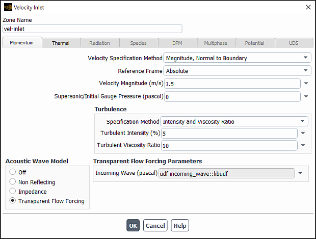
The transparent flow forcing (TFF) boundary condition is available at velocity inlets, mass-flow inlets, pressure inlets, and pressure outlets when simulating transient compressible flow using the pressure-based solver. The steps for using the transparent flow forcing boundary condition are as follows:
Create a profile for the incoming wave intensity on the boundary. The profile can be created either as a profile file as described in Profiles or using the
DEFINE_PROFILEmacro as described in Fluent Customization Manual. In the profile definition, you will specify the wave intensity as a function of position and time. For the incoming wave, the pressure and normal velocity perturbations satisfy the relation:Using this relation the incoming wave intensity at the boundary can be computed from any of the flow perturbation quantities.
where
 is the speed of sound and
  is the acoustic impedance.
Open the boundary condition settings dialog box for the boundary zone of interest (Setting Cell Zone and Boundary Conditions).
On the Momentum tab, select Transparent Flow Forcing under Acoustic Wave Model.
Under Transparent Flow Forcing Parameters, select your profile from the drop-down list next to Incoming Wave.


Important:
If flow is tangential to the boundary, then specify either From Neighboring Cell or Direction Vector for Back flow Direction Specification Method. Do not select Normal to the boundary because this computes the face velocity components from flux to zero values during initialization, which impairs solver convergence.
The TFF condition is implemented on top of the non-reflective boundary condition. Choose a time step size that will not make the CFL number exceed a value of 1 in the cells adjacent to the TFF boundary.
The mean flow in the domain should be well established before enabling TFF.