


Profiles can be boundary conditions, cell zone conditions, and initial conditions for discrete phases. Ansys Fluent provides a very flexible profile definition mechanism. This feature allows you to use experimental data, data calculated by an external program, or data written from a previous solution using the Write Profile Dialog Box (as described in Reading and Writing Profile Files) as the boundary condition for a variable.
Information about profiles is presented in the following subsections:
The following is a list of the six types of profiles that can be read into Ansys Fluent, as well as information about the interpolation method employed by Ansys Fluent for each type.
Point profiles are specified by an unordered set of
 points:
  for 2D problems or
  for 3D problems, where
  . Profiles written using the Write Profile dialog box and profiles of experimental data
in random order are examples of point profiles.
. Profiles written using the Write Profile dialog box and profiles of experimental data
in random order are examples of point profiles.Ansys Fluent will interpolate the point cloud to obtain values at the boundary faces. The default interpolation method for the unstructured point data is zeroth order. That is, for each cell face at the boundary, the solver uses the value from the profile file located closest to the cell. Therefore, to get an accurate specification of an inlet profile using the default interpolation method, your profile file should contain a sufficiently high point density. For information about other available interpolation methods for point profiles, see Using Profiles.
Line profiles are specified for 2D problems by an ordered set of
 points:
  , where
  . Zeroth-order interpolation is performed between the points. An example of a line profile is a profile of
data obtained from an external program that calculates a boundary-layer profile.
. Zeroth-order interpolation is performed between the points. An example of a line profile is a profile of
data obtained from an external program that calculates a boundary-layer profile.Mesh profiles are specified for 3D problems by an
 by
by  mesh of points:
  , where
  and
and  . Zeroth-order interpolation is performed between the points. Examples of mesh profiles are profiles of data
from a structured mesh solution and experimental data in a regular array.
. Zeroth-order interpolation is performed between the points. Examples of mesh profiles are profiles of data
from a structured mesh solution and experimental data in a regular array.Radial profiles are specified for 2D and 3D problems by an ordered set of
 points:
  , where
  . The data in a radial profile are a function of radius only. Linear interpolation is performed between the
points, which must be sorted in ascending order of the
. The data in a radial profile are a function of radius only. Linear interpolation is performed between the
points, which must be sorted in ascending order of the  field. The axis for the cylindrical coordinate system is determined as follows:
For 2D problems, it is the
 -direction vector through (0,0).
For 2D axisymmetric problems, it is the
 -direction vector through (0,0).
For 3D problems involving a swirling fan, it is the fan axis defined in the Fan Dialog Box (unless you are using local cylindrical coordinates at the boundary, as described below).
For 3D problems without a swirling fan, it is the rotation axis of the adjacent fluid zone, as defined in the Fluid Dialog Box (unless you are using local cylindrical coordinates at the boundary, as described below).
For 3D problems in which you are using local cylindrical coordinates to specify conditions at the boundary, it is the axis of the specified local coordinate system.
Axial profiles are specified for 3D problems by an ordered set of
 points:
  , where
  . The data in an axial profile are a function of the axial direction. Linear interpolation is performed
between the points, which must be sorted in ascending order of the
. The data in an axial profile are a function of the axial direction. Linear interpolation is performed
between the points, which must be sorted in ascending order of the  field.
Transient profiles are specified for 2D and 3D profiles by an ordered set of
 points:
  . Linear interpolations are done between the points which must be sorted in ascending order of the
 (time or crank angle) field. Examples of transient profiles are transient cell zone and boundary conditions
(see Transient Cell Zone and Boundary Conditions) and point properties for particle injections (see Point Properties for Transient Injections).
(time or crank angle) field. Examples of transient profiles are transient cell zone and boundary conditions
(see Transient Cell Zone and Boundary Conditions) and point properties for particle injections (see Point Properties for Transient Injections).
There are two profile format options:
The format of the profile files is fairly simple. The file can contain an arbitrary number of profiles. Each profile consists of
a header that specifies the profile name, profile type (point, line,
mesh, radial, or axial), and number of defining
points, and is followed by an arbitrary number of named “fields”. Some of these fields contain the coordinate points
and the rest contain boundary data.
Important: Keep profile names to 64 characters or less. If the profile name contains more than 64 characters, Fluent truncates the name to the first 64 characters.
All quantities, including coordinate values, must be specified in SI units because Ansys Fluent does not perform unit conversion when reading profile files.
Parentheses are used to delimit profiles and the fields within the profiles. Any combination of tabs, spaces, and newlines can be used to separate elements.
Important: In the general format description below, “ | ” indicates that you should input only
one of the items separated by |’s and “ ... ” indicates a continuation of the
list.
((profile1-name point|line|radial n)
 (field1-name a1 a2 ... an)
 (field2-name b1 b2 ... bn)
.
.
.
 (fieldf-name f1 f2 ... fn))

((profile2-name mesh m n)
  (field1-name  a11 a12 ... a1n
                a21 a22 ... a2n
                .
                .
                .
                am1 am2 ... amn)
.
.
.
(fieldf-name   f11  f12 ... f1n
               f21  f22 ... f2n
               .
               .
               .
               fm1 fm2 ... fmn))
Profile names must have all lowercase letters (for example, name). Uppercase letters in profile names
are not acceptable. Each profile of type point, line, and
mesh must contain fields with names x, y, and, for 3D,
z. Each profile of type radial must contain a field with name
r. Each profile of type axial must contain a field with name
z. The rest of the names are arbitrary, but must be valid Scheme symbols. For compatibility with
old-style profile files, if the profile type is missing, point is assumed.
A typical usage of a profile file is to specify the profile of the boundary layer at an inlet. For a compressible flow
calculation, this will be done using profiles of total pressure,  , and
, and  . For an incompressible flow, it might be preferable to specify the inlet value of streamwise velocity,
together with
. For an incompressible flow, it might be preferable to specify the inlet value of streamwise velocity,
together with  and
and  .
.
Below is an example of a profile file that does this:
((turb-prof point 8)
 (x
     4.00000E+00  4.00000E+00  4.00000E+00  4.00000E+00
     4.00000E+00  4.00000E+00  4.00000E+00  4.00000E+00 )
 (y
     1.06443E-03  3.19485E-03  5.33020E-03  7.47418E-03
     2.90494E-01  3.31222E-01  3.84519E-01  4.57471E-01 )
 (u
     5.47866E+00  6.59870E+00  7.05731E+00  7.40079E+00
     1.01674E+01  1.01656E+01  1.01637E+01  1.01616E+01 )
 (tke
     4.93228E-01  6.19247E-01  5.32680E-01  4.93642E-01
     6.89414E-03  6.89666E-03  6.90015E-03  6.90478E-03 )
 (eps
     1.27713E+02  6.04399E+01  3.31187E+01  2.21535E+01
     9.78365E-03  9.79056E-03  9.80001E-03  9.81265E-03 )
 )
CSV profiles are compatible with spreadsheets and are available for both reading and writing in Fluent. Many profile types can be written in CSV format, including:
Radial
Axial
Point (X, Y, Z)
Transient
Transient-Periodic
If writing a profile using the Write Profile dialog box, you can save the profile in CSV format by saving
with a .csv extension.
Files may also be written by other Ansys products including:
Ansys Mechanical (
EXOPTION
)Ansys CFX (Profile Data Format)
Applications using the .csv profile format include:
Formatting Rules:
CSV profiles must be setup so they can be read and interpreted correctly in Fluent:
The profile file must contain the section identifiers shown in Table 7.4: CSV Profile Section Identifiers . Some of the identifiers are optional because not all profiles will contain these additional fields, and they are noted as such. The ordering presented in the table is the ordering that should be present in the file.
Table 7.4: CSV Profile Section Identifiers
Section Identifiers Remark [Name] The next line should have the profile name. Note- if the profile name has space characters, they will be replaced with '-' (space character is not allowed). (Optional) [Parameters] The next line should list the name of each parameter and its value. Parameters that have units should have the appropriate unit in brackets next to the value of the parameter. (Optional) [Spatial Fields] The next line should list the names and units of the Cartesian coordinate system. This indicates whether the profile is 1D, 2D, or 3D (with the number of values corresponding to the dimensions of the profile). [Data] Data values begin on the next line. (Optional) [Faces] The next lines provide the face-node connectivity that allows for previewing the profile as a surface. After the
[Data]identifier you must label the type of data that you are providing; refer to Table 7.5: Profile Types and the Corresponding Required Field Labels for the correct labels. If Fluent does not find one of the expected labels, the profile read will fail.Table 7.5: Profile Types and the Corresponding Required Field Labels
Profile Type Required Field Label radial radius axial axis point X, Y, Z transient time, angle transient-periodic time-periodic, angle-periodic Important: The following labels are reserved for X-axis functions:
x,y,z,r,time, andangle. If your file contains fields labeled with any of these reserved names, then those fields will be treated as X-axis functions. For fields to be considered as Y-axis functions, you must use names that are not reserved for X-axis functions.If there is an unsupported section identifier, Fluent ignores the section and looks for the
[Name]and[Data]section identifiers.Multiple profiles may be included in a single file.
Important:
Only use commas as value separators. Space characters should not be used as they will confuse external spreadsheet applications.
If a profile contains only
NameandDatafields, only SI values are supported. Quantities cannot be entered with units. However, if your profile contains any of the additional fields, then units must be provided and they are not required to be SI.
CSV Profile File Examples
A file containing one profile:
[Name]
outlet
[Data]
x,y,z,x-velocity
-0.00036448459,0.0068932362,3,0.5
0.0014999653,-0.0090896944,3,0.5
-0.0014358073,-0.0094413245,3,    0.5
0.0022810854,0.014916174,3,0.5
-0.0024638004,0.014873175,3,0.5
-0.0069573424,0.013364096,3,0.5
A file containing two profiles, the first one is spatial (steady-state) and the second is transient.
[Name]
outlet
[Data]
x,y,z,x-velocity
-0.00036448459,0.0068932362,3,0.05
0.0014999653,-0.0090896944,3,0.05

[Name]
transient-temperature
[Data]
time,temperature
1.1,300
1.2,350
1.3,400
A file containing one profile with all the optional fields
# Profile Description
[Name],,,,,,,,
example-profile-name,,,,,,,,
,,,,,,,,
[Parameters],,,,,,,,
example-parameter = value,,,,,,,,
example-parameter2 = value [unit],,,,,,,,
example-parameter3 = value [unit],,,,,,,,
,,,,,,,,
[Spatial Fields],,,,,,,,
Initial X [m], Initial Y [m], Initial Z [m],,,,,,
,,,,,,,,
[Data],,,,,,,,
Initial X [m], Initial Y [m], Initial Z [m], norm meshdisptot x [ ], norm meshdisptot y [ ], norm meshdisptot z [ ], norm imag meshdisptot x [ ], norm imag meshdisptot y [ ], norm imag meshdisptot z [ ]
0.26249194,-0.15531575,-2.57E-02,-0.26383738,-0.27941432,-0.10469795,0.24519758,-1.56E-02,0.88077954
0.26336359,-0.15383309,-2.57E-02,-0.26204233,-0.28049517,-0.12765918,0.23875593,-1.19E-02,0.88023709
0.26452365,-0.15182963,-2.57E-02,-0.25952255,-0.28202344,-0.15844249,0.22989663,-6.86E-03,0.87890624
,,,,,,,,
[Faces],,,,,,,,
175,3045,3016,2790,,,,,
2790,3016,3001,2789,,,,,
2789,3001,2986,2788,,,,,
2788,2986,2971,2787,,,,,
The procedure for using a profile to define a particular cell zone or boundary condition is outlined below.
Create a file that contains the desired profile, following the format described in Profile File Formats.
Read the profile using the button in the Profiles Dialog Box (Figure 7.96: The Profiles Dialog Box)
or the File/Read/Profile... ribbon tab item.
 Setup →
  Cell Zone Conditions →
Profiles... Setup → Boundary Conditions →
Profiles...
Cell Zone Conditions →
Profiles... Setup → Boundary Conditions →
Profiles... File → Read → Profile...
Note that if you use the Profiles dialog box to read a file, and a profile in the file has the same name as an existing profile, the old profile will be overwritten.
If it is a point profile, you can choose the method of interpolation using the Profiles dialog box (Figure 7.96: The Profiles Dialog Box):
Setup → Cell Zone Conditions →
Profiles... Setup → Boundary Conditions →
Profiles...Select the point profile in the Profile selection list. Then select one of the three choices in the Interpolation Method list and click the button. The three choices include:
Constant
This method is zeroth-order interpolation. For each cell face at the boundary, the solver uses the value from the profile file located closest to the cell. Therefore, the accuracy of the interpolated profile will be affected by the density of the data points in your profile file. This is the default interpolation method for point profiles.
Inverse Distance
This method assigns a value to each cell face at the boundary based on weighted contributions from the values in the profile file. The weighting factor is inversely proportional to the distance between the profile point and the cell face center.
Least Squares
This method assigns values to the cell faces at the boundary through a first-order interpolation method that tries to minimizes the sum of the squares of the offsets (residuals) between the profile data points and the cell face centers. The least squares solution is found using Singular Value Decomposition (SVD).
Note: The Inverse Distance and Least Squares profile interpolation methods are not applicable when a profile is attached to cell zones. When the cell face is outside the profile-covered zone, the Inverse Distance and Least Squares profile interpolation methods will be switched to the Constant interpolation method to improve the interpolation robustness.
For information about the interpolation methods employed for other profile types (that is, line, mesh, radial, or axial profiles), see Profile Specification Types.
You can attach a profile to a reference frame so that the profile will rotate according to the reference frame. This can be used to model the clocking effect of a rotor on a stator, for example. Under Reference Frames, select the reference frame to attach the chosen profile to.
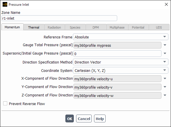
In the boundary conditions dialog boxes (for example, the Velocity Inlet and Pressure Inlet dialog boxes), the fields defined in the profile file (and those defined in any other profile file that you have read in) will appear in the drop-down list to the right of or below each parameter for which profile specification is allowed. To use a particular profile, select it in the appropriate list.
Initialize the solution to interpolate the profile.
Note: You can use a profile file or the DEFINE_PROFILE user-defined function to specify volumetric source terms.
If you specify the source terms with a profile, you will not have access to the central coefficient of the equations solved in
order to linearize the source term. You will need to use a user-defined function to do this.
For more information on UDFs, refer to the Fluent Customization Manual.
Each profile file contains one or more profiles, and each profile has one or more fields defined in it. Once you have read in a profile file, you can check which fields are defined in each profile, and you can also delete a particular profile. These tasks are accomplished in the Profiles Dialog Box (Figure 7.96: The Profiles Dialog Box).
![]() Setup →
Setup → ![]() Cell Zone Conditions →
Profiles...
Cell Zone Conditions →
Profiles...
![]() Setup →
Setup → ![]() Boundary Conditions →
Profiles...
Boundary Conditions →
Profiles...
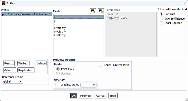
To check which fields are defined in a particular profile, select the profile name in the Profile list. The available fields in that file will be displayed in the Fields list. In Figure 7.96: The Profiles Dialog Box, the profile fields from the profile file of Example are shown.
Any parameters defined within the profile will be listed under Parameters with it's accompanying value.
To delete a profile, select it in the Profile list and click the button. When a profile is deleted, all fields defined in it will be removed from the Fields list.
Important: If you are deleting a profile that is being used as an input for a boundary condition, a cell zone condition, or both, the input will be in a undefined/invalid state after deletion of the profile. To resolve this issue, you must manually update the inputs to a valid input type such as constant, udf/profile, or expression.
If you are deleting an existing profile to replace it with a new profile, use the following procedure:
Delete the existing profile.
Change the parameters defined by the existing profile to Constant.
Read the new profile and apply as desired.
From within Figure 7.96: The Profiles Dialog Box you can preview any profile or profile field as a cloud of points. Additionally, profiles containing node-connectivity data can also be previewed as a surface (profiles that cannot be previewed as a surface are identified in parenthesis in the Profile list).
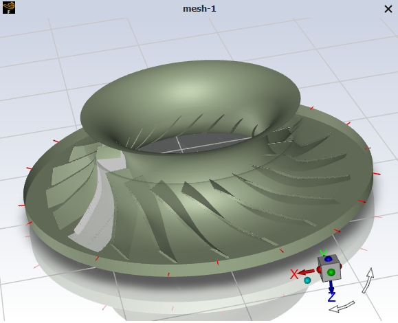
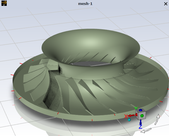
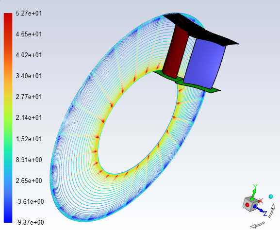
With either type of profile preview, you can include a mesh or contour display by enabling Graphics Object in the Overlay group box and selecting the desired graphics object from the drop-down list. See Figure 7.97: Preview of Profile as a Surface (Gray) with Mesh Overlayed (Pastel Green), Figure 7.98: Preview of Profile as a Point Cloud (Black) with Mesh Overlayed (Pastel Green), and Figure 7.99: Preview of Profile Field as a Point Cloud for examples.
Controls for how the points appear for Point Cloud preview are available by enabling Show Point Properties.
The Plots task page options allow you to generate XY plots of data related to profiles. You can plot the original data points from the profile file you have read into Ansys Fluent, or you can plot the values assigned to the cell faces on the boundary after the profile file has been interpolated. See XY Plots of Profiles for the steps to generate these plots.
You have the additional option of viewing the parameters) using the Plot or the Contours options. Note that these display options do not allow you to plot the actual values of the cell faces (as is done with the Interpolated Data option), because they interpolate the values stored in the adjacent cells. To view the boundary condition parameters you must first read in the profile, save a boundary condition with a profile field selected as a parameter, and initialize the flow solution. Then you can view the surface data as follows:
For 2D calculations, open the Solution XY Plot dialog box. Select the appropriate boundary zone in the Surfaces list, the variable of interest in the Y Axis Function drop-down list, and the desired Plot Direction. Ensure that the check button is turned on, and then click . You should then see the profile plotted. If the data plotted does not agree with your specified profile, this means that there is an error in the profile file.
For 3D calculations, use the Contours dialog box to display contours on the appropriate boundary zone surface. The check button must be turned on in order for you to view the profile data. If the data shown in the contour plot does not agree with your specified profile, this means that there is an error in the profile file.
In Figure 7.100: Example of Using Profiles as Boundary Conditions, profiles are used to specify the gauge total pressure and the x, y, z flow direction components at a pressure inlet boundary.
For 3D cases only, Ansys Fluent allows you to change the orientation of an existing profile so that it can be used at a boundary positioned arbitrarily in space. This allows you, for example, to take experimental data for an inlet with one orientation and apply it to an inlet in your model that has a different spatial orientation. Note that Ansys Fluent assumes that the profile and the boundary are planar.
The procedure for orienting the profile data in the principal directions of a boundary is outlined below:
Define and read the profile as described in Using Profiles.
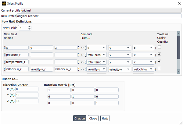
In the Profiles Dialog Box, select the profile in the Profile list, and then click the button. This will open the Orient Profile Dialog Box (Figure 7.101: The Orient Profile Dialog Box).
In the Orient Profile dialog box, enter the name of the new profile you want to create in the New Profile box.
Specify the number of fields you want to create using the up/down arrows next to the New Fields box. The number of new fields is equal to the number of vectors and scalars to be defined plus 1 (for the coordinates).
Define the coordinate field.
Enter the names of the three coordinates (
 ,
,  ,
,  ) in the first row under New Field Names.
Important: Ensure that the coordinates are named
 ,
,  , and
, and  only. Do not use any other names or upper case letters in this field.
Select the appropriate local coordinate fields for
 ,
,  , and
, and  from the drop-down lists under Compute From.... (A selection of
0 indicates that the coordinate does not exist in the original profile; that is, the
original profile was defined in 2D.)
from the drop-down lists under Compute From.... (A selection of
0 indicates that the coordinate does not exist in the original profile; that is, the
original profile was defined in 2D.)
Define the vector fields in the new profile.
Enter the names of the 3 components in the directions of the coordinate axes of the boundary under New Field Names.
Important: Do not use upper case letters in these fields.
Select the names of the 3 components of the vector in the local
 ,
,  , and
, and  directions of the profile from the drop-down lists under Compute
From....
directions of the profile from the drop-down lists under Compute
From....
Define the scalar fields in the new profile.
Enter the name of the scalar in the first column under New Field Names.
Important: Do not use upper case letters in these fields.
Click the button under Treat as Scalar Quantity in the same row.
Select the name of the scalar in the corresponding drop-down list under Compute From....
Under Orient To..., specify the rotational matrix
 under the Rotation Matrix [RM]. The rotational matrix used here is based on
Euler angles (
under the Rotation Matrix [RM]. The rotational matrix used here is based on
Euler angles ( ,
,  , and
, and  ) that define an orthogonal system
  as the result of the three successive rotations from the original system
  . That is,
(7–215)

(7–216)
where C, B, and A are the successive rotations around the
 ,
,  , and
, and  axes, respectively.
Rotation around the
 axis:
axis:
(7–217)
Rotation around the
 axis:
axis:
(7–218)
Rotation around the
 axis:
axis:
(7–219)
Under Orient To..., specify the Direction Vector. The Direction Vector is the vector that translates a profile to the new position, and is defined between the centers of the profile fields.
Important: Note that depending on your case, it may be necessary to perform only a rotation, only a translation, or a combination of a translation and a rotation.
Click the button in the Orient Profile dialog box, and your new profile will be created. Its name, which you entered in the New Profile box, will now appear in the Profiles dialog box and will be available for use at the desired boundary.
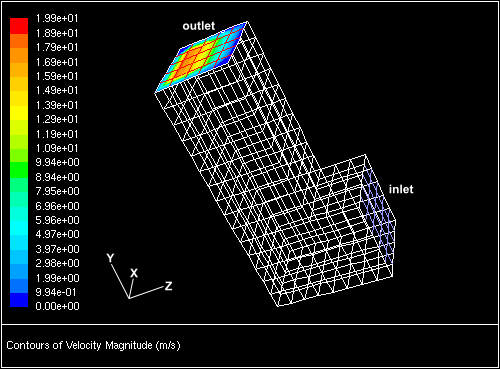
Consider the domain with a square inlet and outlet, shown in Figure 7.102: Scalar Profile at the Outlet. A scalar profile
at the outlet is written out to a profile file. The purpose of this example is to impose this outlet profile on the inlet
boundary via a 90 ° rotation about the  axis. However, the rotation will locate the profile away from the inlet boundary. To align the profile to
the inlet boundary, a translation via a directional vector must be performed.
axis. However, the rotation will locate the profile away from the inlet boundary. To align the profile to
the inlet boundary, a translation via a directional vector must be performed.
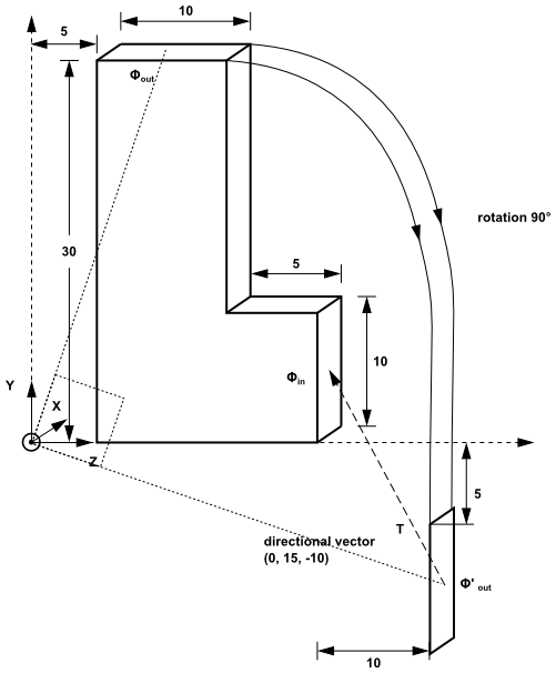
The problem is shown schematically in Figure 7.103: Problem Specification.  is the scalar profile of the outlet.
  is the image of the
  rotated 90 ° around the
  axis. In this example, since
  , then
  , where
  is the identity matrix, and the rotation matrix is
 | (7–220) |
To overlay the outlet profile on the inlet boundary, a translation will be performed.
To overlay the outlet profile on the inlet boundary, a translation will be performed. The directional vector is the vector
that translates  to
to  . In this example, the directional vector is
  . The appropriate inputs for the Orient Profile dialog box are shown in Figure 7.101: The Orient Profile Dialog Box.
Note that if the profile being imposed on the inlet boundary was due to a rotation of -90 °
about the  axis, then the rotational matrix
  must be found for
  and
and  , and a new directional vector must be found to align the profile to the boundary.
In many turbomachinery cases, a profile can be obtained from an initial small-scale simulation (often one passage but sometimes more) and then applied to a larger, often full 360 degree, simulation. Replicating a profile enables you to copy the initial profile periodically for use in a larger simulation.
The following topics are discussed:
The procedure for replicating the profile data periodically is outlined below:
Define and read the profile as described in Using Profiles.
Open the Profiles dialog box.
Physics → Zones →
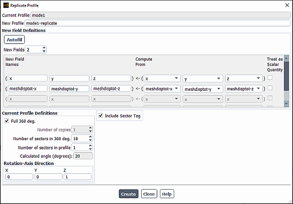
Profiles...Select the profile to replicate and click Replicate... to open the Replicate Profile dialog box (Figure 7.104: The Replicate Profile Dialog Box).
Enter a name in the New Profile field (for the expanded profile name).
If the profile contains mesh displacement field variables (variables containing the
meshdisp,meshdisptotkeyword), the Autofill button becomes available. Upon clicking Autofill, Fluent will automatically fill the dialog box based on the current profile. Otherwise, you can follow the steps below to specify profile replication manually.Specify the number of fields you want to create using the up/down arrows next to the New Fields box. The number of new fields is equal to the number of vectors and scalars to be defined plus 1 (including the coordinates).
Define the coordinate field.
Enter the names of the three coordinates (x, y, z) in the first row under New Field Names.
Important: Ensure that the coordinates are named x, y, and z only. Do not use any other names or upper case letters in this field.
Select the appropriate local coordinate fields for x, y, and z from the drop-down lists under Compute From.... (A selection of 0 indicates that the coordinate does not exist in the original profile; that is, the original profile was defined in 2D.)
Define the vector fields in the new profile.
Enter the names of the 3 components in the directions of the coordinate axes under New Field Names.
Important: Do not use upper case letters in these fields.
Select the names of the 3 components of the vector in the local coordinates of the profile from the drop-down lists under Compute From....
Define the scalar fields in the new profile.
Enter the name of the scalar in the first column under New Field Names.
Important: Do not use upper case letters in these fields.
Select Treat as Scalar Quantity in the same row.
Select the name of the scalar in the corresponding drop-down list under Compute From....
Specify the replication settings in the Current Profile Definitions group box.
If you are creating a full 360 degree profile, select Full 360 deg.. Fluent automatically determines the number of copies of the original profile that are needed to make the full 360 degree profile based on the other information you specify.
If you did not select Full 360 deg., you must specify the Number of copies to manually determine how many copies of the original profile are created.
The Number of sectors in 360 deg. is the number of periodic sections, based on the original profile, that are present in 360 degrees.
The Number of sectors in profile is the number of periodic sections in the original profile.
The Calculated angle is for display only and is the angle occupied by the original profile. When using the Full 360 deg. option, you can determine the number of copies that are created by dividing 360 by the Calculated angle.
Specify the Rotation-Axis Direction. This is the X, Y, and Z components of the axis about which the selected profile is replicated.
Optionally, you can select Include Sector Tag and Fluent will append a sector tag column onto the replicated profile to indicate the original and replicated profiles. The numbering follows the right hand rule applied to the Rotation-Axis Direction that you have specified.
Click the button in the Replicate Profile dialog box, and your new profile will be created. Its name, which you entered in the New Profile box, will now appear in the Profiles dialog box and will be available for use at the desired boundary.
Complex mode shapes are composed of a real and an imaginary vector pair that cannot be replicated (expanded) separately in the same way as is done for other profiles with real-only vectors.
The process of complex mode shape replication is performed as follows:


Where the rotation matrix is  and computed with a given rotation axis
  as:
as:
Note: The rotation matrix is computed in the same way as for non-complex mode shape replication.
 | (7–223) |
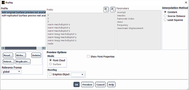
After opening the Replicate Profile dialog box, as described in Replicating Profiles, Fluent detects the presence of a parameter called harmonic index as shown in Figure 7.105: The Profiles Dialog Box with Complex Mode Shape Profile. This parameter must be correctly defined for Fluent to accurately expand the complex
mode shape. Note that the harmonic index parameter is automatically included in profiles generated in Ansys Mechanical for cases
with Cyclic Symmetry. If the profile was created with a source outside of the Ansys environment, you are
responsible for creating the parameter and setting it to the correct value.
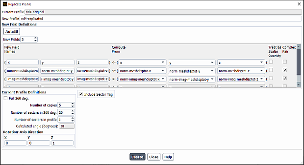
With the presence of the harmonic index parameter, the Replicate Profile
dialog box has an additional column of checkboxes named Complex Pair. Selecting the Complex
Pair checkbox indicates the rows corresponding to the real and imaginary vector pairs of the complex mode
shape, as shown in Figure 7.106: The Replicate Profile Dialog Box with Complex Pair.
The workflow for expanding a complex mode shape is as follows:
Load a profile that contains a parameter named
harmonic index. For details on loading a profile, see Using Profiles.If the profile contains mesh displacement field variables (variables containing the
meshdisp,meshdisptotkeyword), the Autofill button becomes available. Upon clicking Autofill, Fluent will automatically fill the dialog box based on the current profile. Otherwise, you can follow the steps below to specify profile replication manually.Enter the real vector component of the complex mode shape into any row and select Complex Pair. This indicates to Fluent that it is the first part of the complex pair, and that the imaginary vector will immediately follow on the next row.
The real and complex pairs can be defined in any new field row. However, the real vector component must be defined first, followed by the imaginary vector on the immediate row below the real vector.
When the Complex Pair checkbox is selected, the immediate following row will also be set in anticipation of the imaginary vector components being defined. Enter the imaginary vector components in the second row.
Note: When the Complex Pair checkboxes are set, all other checkboxes in that column will be greyed out to prevent another pair from being defined. This is a current limitation that only one complex pair can be defined.
Complete the rest of the dialog box as described in Steps for Replicating a Profile