Periodic flow occurs when the physical geometry of interest and the expected pattern of the flow/thermal solution have a periodically repeating nature. Two types of periodic flow can be modeled in Ansys Fluent. In the first type, no pressure drop occurs across the periodic planes. In the second type, a pressure drop occurs across translationally periodic boundaries, resulting in “fully-developed” or “streamwise-periodic” flow.
This section discusses streamwise-periodic flow. A description of no-pressure-drop periodic flow is provided in Periodic Boundary Conditions, and a description of streamwise-periodic heat transfer is provided in Modeling Periodic Heat Transfer.
Information about streamwise-periodic flow is presented in the following sections:
For more information about the theoretical background of periodic flows, see Periodic Flows in the Theory Guide.
More information about periodic flows is presented in the following sections:
Ansys Fluent provides the ability to calculate streamwise-periodic—or “fully-developed”—fluid flow. These flows are encountered in a variety of applications, including flows in compact heat exchanger channels and flows across tube banks. In such flow configurations, the geometry varies in a repeating manner along the direction of the flow, leading to a periodic fully-developed flow regime in which the flow pattern repeats in successive cycles. Other examples of streamwise-periodic flows include fully-developed flow in pipes and ducts. These periodic conditions are achieved after a sufficient entrance length, which depends on the flow Reynolds number and geometric configuration.
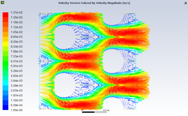
Streamwise-periodic flow conditions exist when the flow pattern repeats over some length
 , with a constant pressure drop across each repeating module along
the streamwise direction. Figure 9.6: Example of Periodic Flow in a 2D Heat Exchanger Geometry depicts one
example of a periodically repeating flow of this type that has been modeled by
including a single representative module. Note that the figure shows the results
plotted for the one periodic pair and two symmetries.
, with a constant pressure drop across each repeating module along
the streamwise direction. Figure 9.6: Example of Periodic Flow in a 2D Heat Exchanger Geometry depicts one
example of a periodically repeating flow of this type that has been modeled by
including a single representative module. Note that the figure shows the results
plotted for the one periodic pair and two symmetries.
The following limitations apply to modeling streamwise-periodic flow:
The flow must be incompressible.
When performing unsteady-state simulations with translational periodic boundary conditions, the specified pressure gradient is recommended.
If one of the density-based solvers is used, you can specify only the pressure jump; for the pressure-based solver, you can specify either the pressure jump or the mass flow rate.
No net mass addition through inlets/exits or extra source terms is allowed.
Species can be modeled only if inlets/exits (without net mass addition) are included in the problem. Reacting flows are not permitted.
When you specify a periodic mass-flow rate, Fluent will assume that the entire flow rate passes through one periodic continuous face zone only. It is not supported to define a mass-flow periodic condition for more than 1 periodic boundary condition (that is, it does not work for 2 periodic pairs).
Steady particle tracks can be modeled only if the particles have a possibility to leave the domain without generating incomplete trajectories.
While multiphase flow can be modeled with translational periodic boundary conditions, you cannot use the mass flow rate specification method. However, you can specify a constant pressure gradient.
For the pressure-based solver, the periodic boundary condition with specified non-zero mass flow rate and/or pressure gradient cannot be used for variable density flows.
For the density-based solver, the periodic pressure jump cannot be used when density is a function of pressure.
When displaying contours of solution variables related to temperature and pressure (such as static temperature, enthalpy, and so on), each nodal value on the periodic boundary is calculated as the weighted average of the values in the cells contacting that node. Since no cells adjacent to the periodic shadow zone contribute to the average, contour values might differ between corresponding places on periodic zones and periodic shadow zones.
For periodic simulations that include heat transfer, see also the limitations described in Constraints for Periodic Heat Transfer Predictions.
Note: The Pressure Gradient refers to the linear component of the calculated pressure gradient.
If you are using the pressure-based solver, in order to calculate a spatially periodic flow field with a specified mass flow rate or pressure derivative, you must first create a mesh with translationally periodic boundaries that are parallel to each other and equal in size. You can specify translational periodicity in the Periodic Conditions Dialog Box, as described in Periodic Boundary Conditions. (If you need to create periodic boundaries, see Creating Periodic Zones and Interfaces).
In the Periodic Conditions Dialog Box that is opened from the Boundary Conditions Task Page, you will complete the following inputs after the mesh has been read into Ansys Fluent (Figure 9.7: The Periodic Conditions Dialog Box):
![]() Setup →
Setup → ![]() Boundary Conditions → Periodic Conditions...
Boundary Conditions → Periodic Conditions...
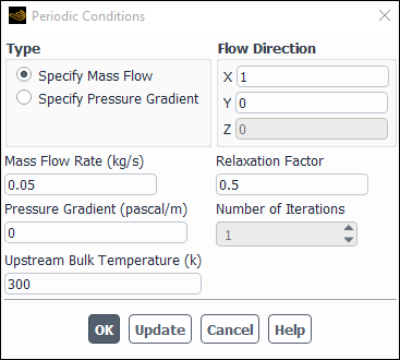
Select either the specified mass flow rate (Specify Mass Flow) option or the specified pressure gradient (Specify Pressure Gradient) option. For most problems, the mass flow rate across the periodic boundary will be a known quantity; for others, the mass flow rate will be unknown, but the pressure gradient (
 in Equation 1–22, in the Theory Guide) will be
a known quantity.
in Equation 1–22, in the Theory Guide) will be
a known quantity.Specify the mass flow rate and/or the pressure gradient (
 in Equation 1–22, in the Theory Guide):
If you selected the Specify Mass Flow option, enter the desired value for the Mass Flow Rate. You can also specify an initial guess for the Pressure Gradient, but this is not required.
Important: For axisymmetric problems, the mass flow rate is per
 radians.
If you selected the Specify Pressure Gradient option, enter the desired value for Pressure Gradient.
Define the flow direction by setting the X,Y,Z (or X,Y in 2D) point under Flow Direction. The flow will move in the direction of the vector pointing from the origin to the specified point. The direction vector must be parallel to the periodic translation direction or its opposite.
If you chose in step 1 to specify the mass flow rate, set the parameters used for the calculation of
 . These parameters are described
in detail below.
. These parameters are described
in detail below.
After completing these inputs, you can solve the periodic velocity field to convergence.
If you choose to specify the mass flow rate, Ansys Fluent must
calculate the appropriate value of the pressure gradient  . You can control this
calculation by specifying the Relaxation Factor and the Number of Iterations, and by supplying
an initial guess for
. You can control this
calculation by specifying the Relaxation Factor and the Number of Iterations, and by supplying
an initial guess for  . All of these inputs are entered in the Periodic Conditions Dialog Box.
The Number of Iterations sets the number
of sub-iterations performed on the correction of  in the pressure correction
equation. Because the value of
in the pressure correction
equation. Because the value of  is not known a priori, it must be iterated
on until the Mass Flow Rate that you have defined
is achieved in the computational model. This correction of
is not known a priori, it must be iterated
on until the Mass Flow Rate that you have defined
is achieved in the computational model. This correction of  occurs in the pressure
correction step of the SIMPLE, SIMPLEC, or PISO algorithm. A correction
to the current value of
occurs in the pressure
correction step of the SIMPLE, SIMPLEC, or PISO algorithm. A correction
to the current value of  is calculated based on the difference between
the desired mass flow rate and the actual one. The sub-iterations
referred to here are performed within the pressure correction step
to improve the correction for
is calculated based on the difference between
the desired mass flow rate and the actual one. The sub-iterations
referred to here are performed within the pressure correction step
to improve the correction for  before the pressure correction equation
is solved for the resulting pressure (and velocity) correction values.
The default value of 2 sub-iterations should suffice in most problems,
but can be increased to help speed convergence. The Relaxation
Factor is an under-relaxation factor that controls convergence
of this iteration process.
before the pressure correction equation
is solved for the resulting pressure (and velocity) correction values.
The default value of 2 sub-iterations should suffice in most problems,
but can be increased to help speed convergence. The Relaxation
Factor is an under-relaxation factor that controls convergence
of this iteration process.
You can also speed up convergence of the periodic calculation
by supplying an initial guess for  in the Pressure
Gradient field. Note that the current value of
in the Pressure
Gradient field. Note that the current value of  will be displayed
in this field if you have performed any calculations. To update the Pressure Gradient field with the current value at any
time, click the button.
will be displayed
in this field if you have performed any calculations. To update the Pressure Gradient field with the current value at any
time, click the button.
If you are using one of the density-based solvers, in order to calculate a spatially periodic flow field with a specified pressure jump, you must first create a mesh with translationally periodic boundaries that are parallel to each other and equal in size. (If you need to create periodic boundaries, see Creating Periodic Zones and Interfaces.)
Then, follow the steps below:
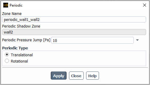
In the Periodic Dialog Box (Figure 9.8: The Periodic Dialog Box), which is opened from the Boundary Conditions task page, indicate that the periodicity is Translational (the default).
 Setup →
  Boundary Conditions →
  Periodic → Edit...
Also in the Periodic Dialog Box, set the Periodic Pressure Jump (
 in Equation 1–21 in
the Theory Guide).
in Equation 1–21 in
the Theory Guide).
After completing these inputs, you can solve the periodic velocity field to convergence.
If you have specified the mass flow rate, you can monitor the value of the pressure gradient
 during the calculation by creating a report plot that includes
periodic pressure gradient, to ensure that you reach a converged solution. See Monitoring Statistics for additional information.
during the calculation by creating a report plot that includes
periodic pressure gradient, to ensure that you reach a converged solution. See Monitoring Statistics for additional information.
Note: Contours of Pressure Gradient are represented by an auxiliary pressure field used by the solver and does not represent a real value.
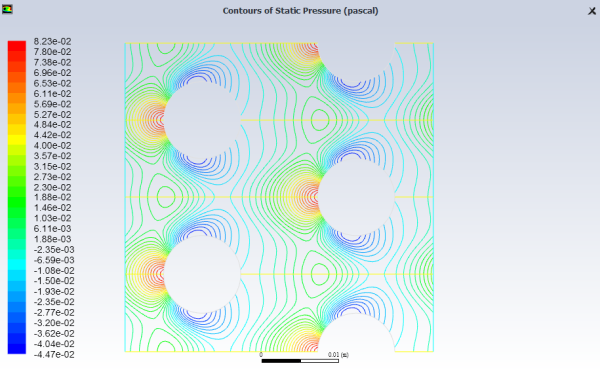
For streamwise-periodic flows, the velocity field should be completely periodic. If a
density-based solver is used to compute the periodic flow, only the linear component of
the pressure field will be reported (which is not periodic). If the pressure-based
solver is used, the pressure field reported will be the periodic pressure field
 of Equation 1–22, in
the Theory Guide. Figure 9.9: Periodic Pressure Field Predicted for Flow in a 2D Heat Exchanger
Geometry displays the periodic pressure field in the
geometry of Figure 9.6: Example of Periodic Flow in a 2D Heat Exchanger Geometry.
of Equation 1–22, in
the Theory Guide. Figure 9.9: Periodic Pressure Field Predicted for Flow in a 2D Heat Exchanger
Geometry displays the periodic pressure field in the
geometry of Figure 9.6: Example of Periodic Flow in a 2D Heat Exchanger Geometry.
If you specified a mass flow rate and had Ansys Fluent calculate
the pressure gradient, you can check the pressure gradient in the
streamwise direction ( ) by looking at the current value for Pressure Gradient in the Periodic Conditions Dialog Box.