


A buoyancy-driven flow is induced due to the force of gravity acting on the density variations. When the density variation is caused by temperature, such buoyancy-driven flows are termed as natural convection flows.
For more information about the theory behind natural convection and buoyancy-driven flows, see Natural Convection and Buoyancy-Driven Flows Theory in the Theory Guide.
When you model natural convection inside a closed domain, the solution will depend on the mass inside the domain. Since this mass will not be known unless the density is known, you must model the flow in one of the following ways:
Perform a transient calculation. In this approach, the initial density will be computed from the initial pressure and temperature, so the initial mass is known. As the solution progresses over time, this mass will be properly conserved. If the temperature differences in your domain are large, you must follow this approach.
Perform a steady-state calculation using the Boussinesq model (described in The Boussinesq Model ). In this approach, you will specify a constant density, so the mass is properly specified. This approach is valid only if the temperature differences in the domain are small. If not, you use the transient approach.
Important: For a closed domain, you can use the incompressible ideal gas law only with a fixed operating pressure. It cannot be used with a floating operating pressure. You can use the compressible ideal or real gas law with either floating or fixed operating pressure.
See Floating Operating Pressure for more information about the floating operating pressure option.
For many natural-convection flows, you can get faster convergence with the Boussinesq model than you can get by setting up the problem with fluid density as a function of temperature. This model treats density as a constant value in all solved equations, except for the buoyancy term in the momentum equation:
 | (7–67) |
where  is the (constant) density of the flow,
  is the operating temperature, and
  is the thermal expansion coefficient. Equation 7–67 is obtained by using the Boussinesq
approximation
is the thermal expansion coefficient. Equation 7–67 is obtained by using the Boussinesq
approximation  to eliminate
  from the buoyancy term. This approximation is accurate as long as changes in actual density are small;
specifically, the Boussinesq approximation is valid when
from the buoyancy term. This approximation is accurate as long as changes in actual density are small;
specifically, the Boussinesq approximation is valid when  .
.
The Boussinesq model should not be used if the temperature differences in the domain are large. In addition, it cannot be used with species calculations, combustion, or reacting flows.
The procedure for including buoyancy forces in the simulation of mixed or natural convection flows is described below.
To activate the calculation of heat transfer, enable the energy equation by right-clicking Energy in the tree (under Setup/Models) and clicking On in the menu that opens (Figure 16.1: Enabling the Energy Equation).
 Setup → Models → Energy
 On
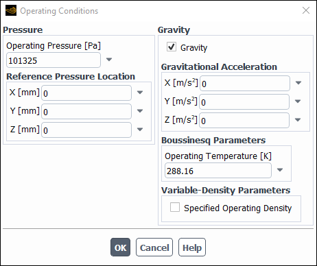
OnDefine the operating conditions in the Operating Conditions dialog box (Figure 7.33: The Operating Conditions Dialog Box).
Setup →  Cell Zone Conditions →
Operating Conditions...
Cell Zone Conditions →
Operating Conditions...Enable the Gravity option under Gravity.
Enter the appropriate values in the X, Y, and (for 3D) Z fields for Gravitational Acceleration for each Cartesian coordinate direction. (Note that the default gravitational acceleration in Ansys Fluent is zero.)
If you are using the incompressible ideal gas law, check that the Operating Pressure is set to an appropriate (nonzero) value.
Depending on whether or not you use the Boussinesq approximation, specify the appropriate parameters described below:
If you are not using the Boussinesq model, the inputs are as follows:
If necessary, define the operating density:
For a single-phase flow, enable the Specified Operating Density option in the Operating Conditions dialog box, and enter a value for the Operating Density. See below for details.
Note: For compressible (ideal and real) gas models with buoyancy, you should specify a value of zero for Operating Density.
For a multiphase flow, Ansys Fluent uses the minimum-phase-averaged operating density method by default. If you want to provide your own input, select the user-input method from the Operating Density drop-down list in the Operating Conditions dialog box (Variable-Density Parameters group box) and enter the value of the operating density. See Setting the Operating Density for a Buoyancy-Driven Multiphase Flow for details.
Define the fluid density as a function of temperature as described in Defining Properties Using Temperature-Dependent Functions and Density.
Setup →
Materials
If you are using the Boussinesq model (described in The Boussinesq Model) the inputs are as follows:
Enter the Operating Temperature (
 in Equation 7–67) in the Operating
Conditions dialog box.
in Equation 7–67) in the Operating
Conditions dialog box.Select boussinesq in the drop-down list for Density in the Create/Edit Materials dialog box as described in Defining Properties Using Temperature-Dependent Functions and Density, and enter a constant value.
Also in the Create/Edit Materials dialog box, enter an appropriate value for the Thermal Expansion Coefficient (
 in Equation 7–67) for the fluid material.
Note that if your model involves multiple fluid materials you can choose whether or not to use the Boussinesq model for each material. As a result, you may have some materials using the Boussinesq model and others not. In such cases, you will need to set all the parameters described above in this step.
Define the boundary conditions. The boundary condition dialog boxes can be opened by right-clicking the boundary name in the tree (under Setup/Boundary Conditions) and clicking Edit... in the menu that opens; alternatively, you can open them from the Boundary Conditions task page:
Setup → Boundary ConditionsThe boundary pressures that you specify at pressure inlet and outlet boundaries are the redefined pressures as given by Equation 7–68. In general you should enter equal pressures,
 , at the inlet and exit boundaries of your Ansys Fluent model if there are no externally imposed
pressure gradients.
, at the inlet and exit boundaries of your Ansys Fluent model if there are no externally imposed
pressure gradients.Set the parameters that control the solution, using the Solution Methods task page.
Solution → MethodsIf you are using the pressure-based solver, selecting PRESTO! for Pressure under Spatial Discretization is recommended.
Add cells near the walls to resolve boundary layers, if necessary.
See also Solving Heat Transfer Problems for information on setting up heat transfer calculations.
When the Boussinesq approximation is not used, the operating density  appears in the body-force term in the momentum equations as
  . This form of the body-force term follows from the redefinition of pressure in Ansys Fluent as
 | (7–68) |
The hydrostatic pressure in a fluid at rest is then
 | (7–69) |
By default, Ansys Fluent will compute the operating density by averaging over all cells. In some cases, you may obtain
better results if you explicitly specify the operating density instead of having the solver compute it for you. For example,
if you are solving a natural-convection problem with a pressure boundary, it is important to understand that the pressure you
are specifying is  in Equation 7–68. Although you will know the actual pressure
  , you will need to know the operating density
  in order to determine
  from
from  . Therefore, you should explicitly specify the operating density rather than use the computed average. The
specified value should, however, be representative of the average value.
. Therefore, you should explicitly specify the operating density rather than use the computed average. The
specified value should, however, be representative of the average value.
In some cases the specification of an operating density will improve convergence behavior, rather than the actual results. For such cases use the approximate bulk density value as the operating density and be sure that the value you choose is appropriate for the characteristic temperature in the domain.
Note that if you are using the Boussinesq approximation for all fluid materials, the operating density  does not appear in the body-force term of the momentum equation. Consequently, you need not specify
it.
does not appear in the body-force term of the momentum equation. Consequently, you need not specify
it.
Details on setting the operation density for multiphase flows can be found in Modeling Buoyancy-Driven Multiphase Flow.
For high-Rayleigh-number flows you may want to consider the solution guidelines below. In addition, the guidelines presented in Solution Strategies for Heat Transfer Modeling for solving other heat transfer problems can also be applied to buoyancy-driven flows. No steady-state solution exists for some laminar, high-Rayleigh-number flows.
When you are solving a high-Rayleigh-number flow ( ), you should follow one of the procedures outlined below for best results.
The first procedure uses a steady-state approach:
Start the solution with a lower value of Rayleigh number (for example,
 ) and run it to convergence using the first-order scheme.
To change the effective Rayleigh number, change the value of gravitational acceleration (for example, from 9.8 to 0.098 to reduce the Rayleigh number by two orders of magnitude).
Use the resulting data file as an initial guess for the higher Rayleigh number and start the higher-Rayleigh-number solution using the first-order scheme.
After you obtain a solution with the first-order scheme you may continue the calculation with a higher-order scheme.
The second procedure uses a time-dependent approach to obtain a steady-state solution [62]:
Start the solution from a steady-state solution obtained for the same or a lower Rayleigh number.
Estimate the time constant as [17]

(7–70)
where
 and
and  are the length and velocity scales, respectively. Use a time step size
  such that
(7–71)
Using a larger time step size may lead to divergence.
After oscillations with a typical frequency of
 0.05–0.09 have decayed, the solution reaches steady-state. Note that
  is the time constant estimated in Equation 7–70 and
  is the oscillation frequency in Hz. In general this solution process may take as many as 5000 time
steps to reach steady-state.
is the oscillation frequency in Hz. In general this solution process may take as many as 5000 time
steps to reach steady-state.