


Material properties can be defined as functions of temperature. For most properties, you can define a polynomial, piecewise-linear, or piecewise-polynomial function of temperature. For specific heat (Cp), you can also use a nasa-9-piecewise-polynomial function of temperature in extremely high-temperature applications. The definitions of these functions are as follows:


In the equations above,  is the property.
Important: If you define a polynomial or piecewise-polynomial function of temperature, the temperature in the function is always in units of Kelvin or Rankine. If you use Celsius or Kelvin as the temperature unit, then polynomial coefficient values must be entered in terms of Kelvin. If you use Fahrenheit or Rankine as the temperature unit, enter the values in terms of Rankine.
Some properties have additional functions available and for some only a subset of these three functions can be used. See the section on the property in question to determine which temperature-dependent functions you can use.
For additional information, see the following sections:
To define a polynomial function of temperature for a material property, do the following:
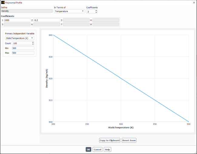
In the Create/Edit Materials Dialog Box, choose polynomial in the drop-down list to the right of the property name (for example, Density). The Polynomial Profile Dialog Box (Figure 8.12: The Polynomial Profile Dialog Box) will open automatically.
Since this is a modal dialog box, the solver will not allow you to do anything else until you perform the following steps.
Specify the number of Coefficients up to 8 coefficients are available. The number of coefficients defines the order of the polynomial. The default of 1 defines a polynomial of order 0. The property will be constant and equal to the single coefficient
 . An input
of 2 defines a polynomial of order 1 and the property will vary linearly
with temperature and so on.
. An input
of 2 defines a polynomial of order 1 and the property will vary linearly
with temperature and so on.Define the coefficients. Coefficients 1, 2, 3,... correspond to
 ,
,  ,
,  ,... in Equation 8–1. The
dialog box in Figure 8.12: The Polynomial Profile Dialog Box shows the
inputs for the following function:
,... in Equation 8–1. The
dialog box in Figure 8.12: The Polynomial Profile Dialog Box shows the
inputs for the following function:
(8–5)
To visualize your profile, ensure the correct Primary Independent Variable is selected from the drop-down list, and enter a value for the Min and Max.
Important: To ensure the robustness of simulations when using polynomials to specify material property, set the solution limits so that the values returned by the polynomial expression are physically valid. For example, when the density of a material is specified as a function of temperature using a polynomial expression, set the proper limits on the temperature range so that the density is always non-negative. For more information on setting solution limits see Setting Solution Limits.
Also, note the restriction on the units for temperature, as described in the previous section.
To define a piecewise-linear function of temperature for a material property, do the following:
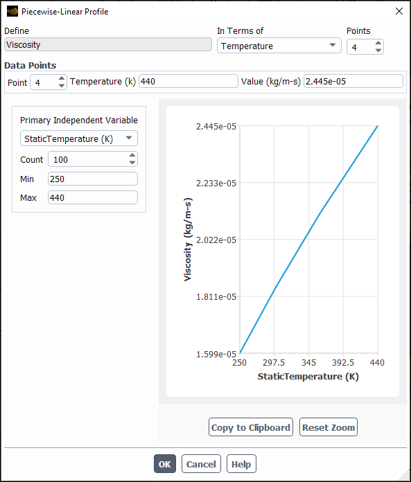
In the Create/Edit Materials Dialog Box, choose piecewise-linear in the drop-down list to the right of the property name (for example, Viscosity). The Piecewise-Linear Profile Dialog Box (Figure 8.13: The Piecewise-Linear Profile Dialog Box) will open automatically.
Since this is a modal dialog box, the solver will not allow you to do anything else until you perform the following steps.
Set the number of Points defining the piecewise distribution.
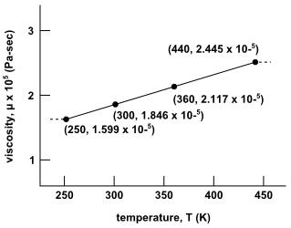
Under Data Points, enter the data pairs for each point. First enter the independent and dependent variable values for Point 1, then increase the Point number and enter the appropriate values for each additional pair of variables. The pairs of points must be supplied in the order of increasing value of temperature. The solver will not sort them for you. A maximum of 50 piecewise points can be defined for each property. The dialog box in Figure 8.13: The Piecewise-Linear Profile Dialog Box shows the final inputs and a plot of the profile that is depicted in Figure 8.14: Piecewise-Linear Definition of Viscosity as a Function of Temperature.
Important: If the temperature exceeds the maximum Temperature (
 )
you have specified for the profile, Ansys Fluent will use the Value corresponding to
)
you have specified for the profile, Ansys Fluent will use the Value corresponding to  . If the temperature falls below the minimum Temperature (
 )
specified for your profile, Ansys Fluent will use the Value corresponding to
)
specified for your profile, Ansys Fluent will use the Value corresponding to  .
.To visualize your profile, ensure the correct Primary Independent Variable is selected from the drop-down list, and enter a value for the Min and Max.
To define a piecewise-polynomial function of temperature for a material property, follow these steps:
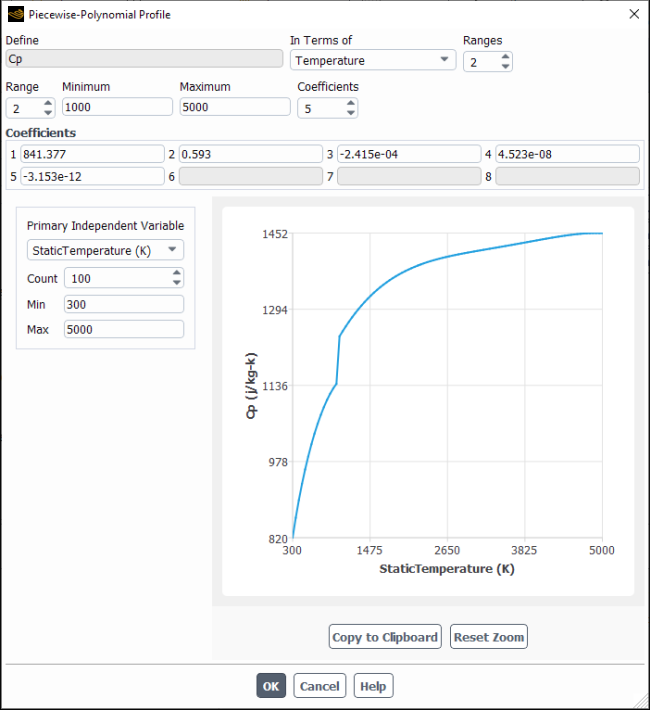
In the Create/Edit Materials Dialog Box, choose piecewise-polynomial in the drop-down list to the right of the property name (for example, Cp). The Piecewise-Polynomial Profile Dialog Box (Figure 8.15: The Piecewise-Polynomial Profile Dialog Box) will open automatically. Since this is a modal dialog box, first perform the following steps.
Specify the number of Ranges. For the example of Equation 8–6, two ranges of temperatures are defined:

(8–6)
You may define up to three ranges. The ranges must be supplied in the order of increasing value of temperature. The solver will not sort them for you.
For the first range (Range = 1), specify the Minimum and Maximum temperatures, and the number of Coefficients. (Up to eight coefficients are available.) The number of coefficients defines the order of the polynomial. The default of
1defines a polynomial of order 0. The property will be constant and equal to the single coefficient . An input
of
. An input
of 2defines a polynomial of order 1. The property will vary linearly with temperature and so on.Define the coefficients. Coefficients 1, 2, 3,... correspond to
 ,
,  ,
,  ,... in Equation 8–3. The dialog box in
Figure 8.15: The Piecewise-Polynomial Profile Dialog Box shows the inputs for the first
range of Equation 8–6.
,... in Equation 8–3. The dialog box in
Figure 8.15: The Piecewise-Polynomial Profile Dialog Box shows the inputs for the first
range of Equation 8–6.Increase the value of Range and enter the Minimum and Maximum temperatures, number of Coefficients, and the Coefficients (
 ,
,  ,
,  ,...) for the
next range. Repeat if there is a third range.
,...) for the
next range. Repeat if there is a third range.To visualize your profile, ensure the correct Primary Independent Variable is selected from the drop-down list, and enter a value for the Min and Max.
This function is available for specific heat only and is useful for hypersonic flows, and can be used with the two-temperature model, where piecewise-polynomial temperature profiles are not valid.
The procedure for defining a nasa-9-piecewise-polynomial function of temperature is similar to that for the piecewise-polynomial function:
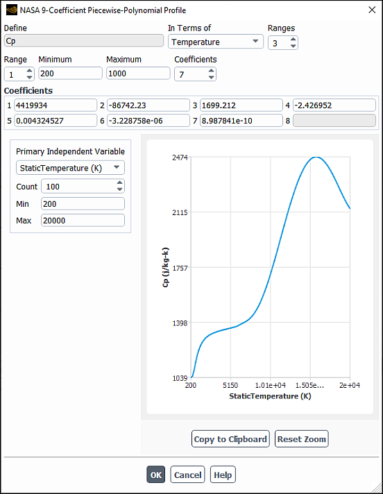
In the Create/Edit Materials Dialog Box, choose nasa-9-piecewise-polynomial from the Cp (Specific Heat) drop-down list (Properties group box). The NASA-9-Coefficient Piecewise-Polynomial Profile dialog box opens automatically with Cp and Temperature displayed in the Define and In Terms of fields, respectively (see Figure 8.16: The NASA-9-Coefficient Piecewise-Polynomial Profile Dialog Box). Note that because this is a modal dialog box, you must tend to it immediately.
Specify the number of Ranges.
You may define up to eight ranges. The ranges must be supplied in the order of increasing value of temperature. The solver will not sort them for you.
For the first range (Range = 1) specify:
The Minimum and Maximum temperatures
The number of Coefficients
Up to eight coefficients are available
Coefficients 1, 2, 3, and so on.
Coefficients 1, 2, 3,... correspond to
, , ,…, respectively, in Equation 8–4.
To visualize your profile, enter a value for the Min and Max. Note that Static Temperature is automatically selected from the Primary Independent Variable drop-down list. You can increase or decrease the value of Count to control the smoothness of the profile curve. You can click and drag in the plot to change the zoom level.
Increase the value of Range and enter the Minimum and Maximum temperatures, number of Coefficients, and their values (
, , , and so on) for the next range.Repeat the previous step for every range if there are more than two ranges.
If you want to check or change the coefficients, data pairs, or ranges for a previously-defined profile, click the button to the right of the property name. The appropriate dialog box will open, and you can check or modify the inputs as desired.
Important: In the Fluent Database Materials Dialog Box, you cannot edit the profiles, but you can examine them by clicking on the button (instead of the button.)