


The macros presented in this section access Ansys Fluent data that you can use in your UDF. Unless indicated, these macros can be used in UDFs for single-phase and multiphase applications.
- 3.2.1. Axisymmetric Considerations for Data Access Macros
- 3.2.2. Node Macros
- 3.2.3. Cell Macros
- 3.2.4. Face Macros
- 3.2.5. Connectivity Macros
- 3.2.6. Special Macros
- 3.2.7. Time-Sampled Data
- 3.2.8. Model-Specific Macros
- 3.2.9. NIST Real Gas Saturation Properties
- 3.2.10. NIST Real Gas UDF Access Macro for Multi-Species Mixtures
- 3.2.11. User-Defined Scalar (UDS) Transport Equation Macros
- 3.2.12. User-Defined Memory (UDM) Macros
C-side calculations for axisymmetric models in Ansys Fluent are made on a 1 radian
basis. Therefore, when you are utilizing certain data access macros (for example,
F_AREA or F_FLUX) for axisymmetric
flows, your UDF will need to multiply the result by 2*PI (utilizing the macro M_PI) to get
the desired value.
A mesh in Ansys Fluent is defined by the position of its nodes and how the nodes are
connected. The macros listed in Table 3.1: Macros for Node Coordinates Defined in metric.h
and Table 3.2: Macro for Number of Nodes Defined in mem.h
can be used to return the real
Cartesian coordinates of the cell node (at the cell corner) in SI units. The variables are
available in both the pressure-based and the density-based solvers. Definitions for these
macros can be found in metric.h. The argument Node
*node for each of the variables defines a node.
Table 3.1: Macros for Node Coordinates Defined in metric.h
|
Macro |
Argument Types |
Returns |
|---|---|---|
|
|
|
|
|
|
|
|
|
|
|
|
The macro F_NNODES shown in Table 3.2: Macro for Number of Nodes Defined in mem.h
returns the integer number of nodes associated with a
face.
Table 3.2: Macro for Number of Nodes Defined in mem.h
|
Macro |
Argument Types |
Returns |
|---|---|---|
|
|
|
|
The macros listed in Table 3.3: Macro for Cell Centroids Defined in metric.h
– Table 3.20: Macros for Multiphase Variables Defined in sg_mphase.h
can be used to return real cell
variables in SI units. They are identified by the C_ prefix. These
variables are available in the pressure-based and the density-based solvers. The quantities
that are returned are available only if the corresponding physical model is active. For
example, species mass fraction is available only if species transport has been enabled in
the Species Model dialog box in Ansys Fluent. Definitions for these macros
can be found in the referenced header file (for example, mem.h).
The macro listed in Table 3.3: Macro for Cell Centroids Defined in metric.h
can be used to obtain the
real centroid of a cell. C_CENTROID
finds the coordinate position of the centroid of the cell c and
stores the coordinates in the x array. Note that the
x array is always one-dimensional, but it can be
x[2] or x[3] depending on whether you
are using the 2D or 3D solver.
Table 3.3: Macro for Cell Centroids Defined in metric.h
|
Macro |
Argument Types |
Outputs |
|---|---|---|
|
|
|
|
See
DEFINE_INIT
for an example UDF that utilizes
C_CENTROID.
The macro listed in Table 3.4: Macro for Cell Volume Defined in mem.h
can be used to obtain the
real cell volume for 2D, 3D, and axisymmetric
simulations.
Table 3.4: Macro for Cell Volume Defined in mem.h
|
Macro |
Argument Types |
Returns |
|---|---|---|
|
|
|
|
See
DEFINE_UDS_UNSTEADY
C_VOLUME.
The macro C_NFACES shown in Table 3.5: Macros for Number of Node and Faces Defined in mem.h
returns the integer number of faces for a given cell.
C_NNODES, also shown in Table 3.2: Macro for Number of Nodes Defined in mem.h
,
returns the integer number of nodes for a given cell.
Table 3.5: Macros for Number of Node and Faces Defined in mem.h
|
Macro |
Argument Types |
Returns |
|---|---|---|
|
|
|
|
|
|
|
|
C_FACE expands to return the global face index face_t
f for the given cell_t c, Thread
*t, and local face index number i. Specific faces
can be accessed via the integer index i and all faces can be
looped over with c_face_loop. The macro is defined in
mem.h.
Note: If you are running in parallel, C_FACE expands to return
the local face index for a compute node.
Table 3.6: Macro for Cell Face Index Defined in mem.h
|
Macro |
Argument Types |
Returns |
|---|---|---|
|
|
|
global face index |
C_FACE_THREAD expands to return the Thread
*t of the face_t f that is returned by
C_FACE (see above). Specific faces can be accessed via the
integer index i and all faces can be looped over with
c_face_loop. The macro is defined in
mem.h.
Table 3.7: Macro for Cell Face Index Defined in mem.h
|
Macro |
Argument Types |
Returns |
|---|---|---|
|
|
|
|
You can access flow variables using macros listed in Table 3.8: Macros for Cell Flow Variables Defined in mem.h or sg_mem.h.
Table 3.8: Macros for Cell Flow Variables Defined in mem.h or sg_mem.h
|
Macro |
Argument Types |
Returns |
|---|---|---|
|
|
|
density |
|
|
|
pressure |
|
|
|
u velocity |
|
|
|
v velocity |
|
|
|
w velocity |
|
|
|
temperature |
|
|
|
enthalpy |
|
|
|
turb. kinetic energy |
|
|
|
turbulent viscosity for Spalart-Allmaras |
|
|
|
turb. kinetic energy dissipation rate |
|
|
|
specific dissipation rate |
|
|
Note: |
species mass fraction |
|
|
|
ignition mass fraction |
|
|
|
premixed combustion temperature |
|
|
|
value of variable |
Note: The C_YI(c,t,i) macro is not available with the
non/partially premixed models. See Species Fractions Calculations with the Non- and Partially- Premixed Models for Information on
calculating the species fractions with the non-premixed and partially premixed
models.
Table 3.9: Macro for Cell Porosity in mem.h
|
Macro |
Argument Types |
Returns |
|---|---|---|
|
|
|
porosity of fluid cell |
|
|
|
porosity of fluid at the dual cell zone region in the non-equilibrium thermal model[a] |
[a] see  in Equation 7–15 in the Fluent User's Guide.
When the non-premixed or partially premixed model is enabled, Ansys Fluent uses lookup
tables to calculate temperature, density, and species fractions. If you need to access
these variables in your UDF, then note that while density and temperature can be
obtained through the macros C_R(c,t) and
C_T(c,t), if you need to access the species fractions, you
will need to first retrieve them by calling the species lookup functions
Pdf_Yi(c, t, n) or Pdf_XY(c,t,x,y).
The functions are defined in the header file pdf_props.h, which you
will need to include in your UDF:
Pdf_XY returns the species mole and mass fraction arrays x and
y.
|
Function: |
|
Argument Type |
Description |
|---|---|
|
|
Cell index. |
|
|
Pointer to thread. |
|
|
Array of species mole fractions. |
|
|
Array of species mass fractions. |
Function returns
void
Pdf_Yi returns the mass fraction of species n.
|
Function: |
|
Argument Type |
Description |
|---|---|
|
|
Cell index. |
|
|
Pointer to thread. |
|
|
Species index. |
Function returns
real
The species number in the lookup tables is stored in the integer variable
n_spe_pdf, which is also included in the header file
pdf_props.h.
You can access gradient and reconstruction gradient vectors (and components) for many
of the cell variables listed in Table 3.8: Macros for Cell Flow Variables Defined in mem.h or
sg_mem.h. Ansys Fluent calculates
the gradient of flow in a cell (based on the divergence theory) and stores this value in
the variable identified by the suffix _G. For example, cell
temperature is stored in the variable C_T, and the temperature
gradient of the cell is stored in C_T_G. The gradients stored in
variables with the _G suffix are non-limited values and if used
to reconstruct values within the cell (at faces, for example), may potentially result in
values that are higher (or lower) than values in the surrounding cells. Therefore, if your
UDF needs to compute face values from cell gradients, you should use the reconstruction
gradient (RG) values instead of non-limited gradient (G) values. Reconstruction gradient
variables are identified by the suffix _RG, and use the limiting
method that you have activated in your Ansys Fluent model to limit the cell gradient
values.
Table 3.10: Macros for Cell Gradients Defined in mem.h
shows a list of cell gradient vector macros. Note
that gradient variables are available only when the equation for that
variable is being solved. For example, if you are defining a source term for energy, your
UDF can access the cell temperature gradient (using C_T_G), but
it cannot get access to the x-velocity gradient (using C_U_G).
The reason for this is that the solver continually removes data from memory that it does
not need. In order to retain the gradient data (when you want to set up user-defined
scalar transport equations, for example), you can prevent the solver from freeing up
memory by enabling the following text command:
solve/set/advanced/retain-temporary-solver-mem. Note that when
you do this, all of the gradient data is retained, but the calculation requires more
memory to run.
You can access a component of a gradient vector by specifying it as an argument in the
gradient vector call (0 for the x component;
1 for y; and 2
for z). For example,
C_T_G(c,t)[0]; /* returns the x-component of the cell temperature gradient vector */
Table 3.10: Macros for Cell Gradients Defined in mem.h
|
Macro |
Argument Types |
Returns |
|---|---|---|
|
|
|
pressure gradient vector |
|
|
|
velocity gradient vector |
|
|
|
velocity gradient vector |
|
|
|
velocity gradient vector |
|
|
|
temperature gradient vector |
|
|
|
enthalpy gradient vector |
|
|
|
turbulent viscosity for Spalart- Allmaras gradient vector |
|
|
|
turbulent kinetic energy gradient vector |
|
|
|
turbulent kinetic energy dissipation rate gradient vector |
|
|
|
specific dissipation rate gradient vector |
|
|
Note: |
species mass fraction gradient vector |
Important: Note that you can access vector components of each of the variables listed in Table 3.10: Macros for Cell Gradients Defined in mem.h
by using the integer index [i]
for each macro listed in Table 3.10: Macros for Cell Gradients Defined in mem.h
. For example,
C_T_G(c,t)[i] will access a component of the temperature
gradient vector.
Important:
C_P_G can be used only in the pressure-based solver.
Important:
C_YI_G can be used only in the density-based solver. To use
this in the pressure-based solver, you will need to set the rpvar
’species/save-gradients? to
#t.
As stated previously, the availability of gradient variables is affected by your
solver selection, which models are turned on, the setting for the spatial discretization,
and whether the temporary solver memory is retained. To make it easy for you to verify
what gradient variables are available for your particular case and data files, the
following UDF (named showgrad.c) is provided. Simply compile this
UDF, run your solution, and then hook the UDF using the Execute on
Demand dialog box (as described in Hooking DEFINE_ON_DEMAND UDFs). The available gradient variables will be displayed in the console.
Important: Note that the showgrad.c UDF is useful only for
single-phase models.
/*
* ON Demand User-Defined Functions to check *
* on the availability of Reconstruction Gradient and Gradients *
* for a given Solver and Solver settings: *
* *
* Availability of Gradients & Reconstruction Gradients depends on: *
* 1) the selected Solver (density based or pressure based) *
* 2) the selected Model *
* 3) the order of discretizations *
* 4) whether the temporary solver memory is being retained (to keep *
* temporary memory, enable the following text command: *
* solve/set/advanced/retain-temporary-solver-mem. *
* *
* *
* How to use showgrad: *
* *
* - Read in your case & data file. *
* - Compile showgrad.c UDF. *
* - Load library libudf. *
* - Attach the showgrad UDF in the Execute on Demand dialog box. *
* - Run your solution. *
* - Click the Execute button in the Execute on Demand dialog box. *
* *
* A list of available Grads and Recon Grads will be displayed in the *
* console. *
* *
* 2004 Laith Zori *
*/ #include "udf.h"
DEFINE_ON_DEMAND(showgrad)
{
Domain *domain;
Thread *t; domain=Get_Domain(1);
if (! Data_Valid_P()) return;
Message0(" >>> entering show-grad: \n ");
thread_loop_c(t, domain)
{
Material *m = THREAD_MATERIAL(t);
int nspe = MIXTURE_NSPECIES(m);
int nspm = nspe-1;
Message0("::::\n ");
Message0(":::: Reconstruction Gradients :::: \n ");
Message0("::::\n ");
if (NNULLP(THREAD_STORAGE(t, SV_P_RG)))
{
Message0("....show-grad:Reconstruction Gradient of P is available \n ");
}
if (NNULLP(THREAD_STORAGE(t, SV_U_RG)))
{
Message0("....show-grad:Reconstruction Gradient of U is available \n ");
}
if (NNULLP(THREAD_STORAGE(t, SV_V_RG)))
{
Message0("....show-grad:Reconstruction Gradient of V is available \n ");
}
if (NNULLP(THREAD_STORAGE(t, SV_W_RG)))
{
Message0("....show-grad:Reconstruction Gradient of W is available \n ");
}
if (NNULLP(THREAD_STORAGE(t, SV_T_RG)))
{
Message0("....show-grad:Reconstruction Gradient of T is available \n ");
}
if (NNULLP(THREAD_STORAGE(t, SV_H_RG)))
{
Message0("....show-grad:Reconstruction Gradient of H is available \n ");
}
if (NNULLP(THREAD_STORAGE(t, SV_K_RG)))
{
Message0("....show-grad:Reconstruction Gradient of K is available \n ");
}
if (NNULLP(THREAD_STORAGE(t, SV_D_RG)))
{
Message0("....show-grad:Reconstruction Gradient of D is available \n ");
}
if (NNULLP(THREAD_STORAGE(t, SV_O_RG)))
{
Message0("....show-grad:Reconstruction Gradient of O is available \n ");
}
if (NNULLP(THREAD_STORAGE(t, SV_NUT_RG)))
{
Message0("....show-grad:Reconstruction Gradient of NUT is available \n ");
}
if (nspe && NNULLP(THREAD_STORAGE(t, SV_Y_RG)))
{
Message0("....show-grad:Reconstruction Gradient of Species is available \n ");
}
/********************************************************************/
/********************************************************************/
/********************************************************************/
/********************************************************************/
Message0("::::\n ");
Message0(":::: Gradients :::: \n ");
Message0("::::\n ");
if (NNULLP(THREAD_STORAGE(t, SV_P_G)))
{
Message0("....show-grad:Gradient of P is available \n ");
}
if (NNULLP(THREAD_STORAGE(t, SV_U_G)))
{
Message0("....show-grad:Gradient of U is available \n ");
}
if (NNULLP(THREAD_STORAGE(t, SV_V_G)))
{
Message0("....show-grad:Gradient of V is available \n ");
}
if (NNULLP(THREAD_STORAGE(t, SV_W_G)))
{
Message0("....show-grad:Gradient of W is available \n ");
}
if (NNULLP(THREAD_STORAGE(t, SV_T_G)))
{
Message0("....show-grad:Gradient of T is available \n ");
}
if (NNULLP(THREAD_STORAGE(t, SV_H_G)))
{
Message0("....show-grad:Gradient of H is available \n ");
}
if (NNULLP(THREAD_STORAGE(t, SV_K_G)))
{
Message0("....show-grad:Gradient of K is available \n ");
}
if (NNULLP(THREAD_STORAGE(t, SV_D_G)))
{
Message0("....show-grad:Gradient of D is available \n ");
}
if (NNULLP(THREAD_STORAGE(t, SV_O_G)))
{
Message0("....show-grad:Gradient of O is available \n ");
}
if (NNULLP(THREAD_STORAGE(t, SV_NUT_G)))
{
Message0("....show-grad:Gradient of NUT is available \n ");
}
if (nspe && NNULLP(THREAD_STORAGE(t, SV_Y_G)))
{
Message0("....show-grad:Gradient of Species is available \n ");
}
}
}
Reconstruction Gradient (RG) Vector Macros
Table 3.11: Macros for Cell Reconstruction Gradients (RG) Defined in mem.h
shows a list of cell reconstruction gradient vector
macros. Like gradient variables, RG variables are available only when the equation for
that variable is being solved. As in the case of gradient variables, you can retain all of
the reconstruction gradient data by enabling the following text command:
solve/set/advanced/retain-temporary-solver-mem. Note that when
you do this, the reconstruction gradient data is retained, but the calculation requires
more memory to run.
You can access a component of a reconstruction gradient vector by specifying it as an
argument in the reconstruction gradient vector call (0 for the
x component; 1 for y;
and 2 for z). For example,
C_T_RG(c,t)[0]; /* returns the x-component of the cell temperature
reconstruction gradient vector */
Table 3.11: Macros for Cell Reconstruction Gradients (RG) Defined in mem.h
|
Macro |
Argument Types |
Returns |
|---|---|---|
|
|
|
density RG vector |
|
|
|
pressure RG vector |
|
|
|
velocity RG vector |
|
|
|
velocity RG vector |
|
|
|
velocity RG vector |
|
|
|
temperature RG vector |
|
|
|
enthalpy RG vector |
|
|
|
turbulent viscosity for Spalart-Allmaras RG vector |
|
|
|
turbulent kinetic energy RG vector |
|
|
|
turbulent kinetic energy dissipation rate RG vector |
|
|
Note: |
species mass fraction RG vector |
Important: Note that you can access vector components by using the integer index
[i] for each macro listed in Table 3.11: Macros for Cell Reconstruction Gradients (RG) Defined in mem.h
. For example, C_T_RG(c,t)[i]
will access a component of the temperature reconstruction gradient vector.
Important:
C_P_RG can be used in the pressure-based solver only when the
second order discretization Scheme for pressure is specified.
Important:
C_YI_RG can be used only in the density-based solver.
As stated previously, the availability of reconstruction gradient variables is affected by your solver selection, which models are turned on, the setting for the spatial discretization, and whether the temporary solver memory is freed. To make it easy for you to verify which reconstruction gradient variables are available for your particular case and data files, a UDF (named showgrad.c) has been provided that will display the available gradients in the console. See the previous section for details.
The _M1 suffix can be applied to some of the cell variable
macros in Table 3.8: Macros for Cell Flow Variables Defined in mem.h or
sg_mem.h to allow access to the value of the
variable at the previous time step (that is,  ). These data may be useful in unsteady simulations. For example,
C_T_M1(c,t);
returns the value of the cell temperature at the previous time step. Previous time step macros are shown in Table 3.12: Macros for Cell Time Level 1 Defined in mem.h .
Important: Note that data from C_T_M1 is available
only if user-defined scalars are defined. It can also be used
with adaptive time stepping.
Table 3.12: Macros for Cell Time Level 1 Defined in mem.h
|
Macro |
Argument Types |
Returns |
|---|---|---|
|
|
|
density, previous time step |
|
|
|
velocity, previous time step |
|
|
|
velocity, previous time step |
|
|
|
velocity, previous time step |
|
|
|
temperature, previous time step |
|
|
Note: |
species mass fraction, previous time step |
See
DEFINE_UDS_UNSTEADY
for an example UDF that utilizes
C_R_M1.
The M2 suffix can be applied to some of the cell variable
macros in Table 3.12: Macros for Cell Time Level 1 Defined in mem.h
to allow access to the value of the
variable at the time step before the previous one (that is,  ). These data may be useful in unsteady simulations. For example,
C_T_M2(c,t);
returns the value of the cell temperature at the time step before the previous one (referred to as second previous time step). Two previous time step macros are shown in Table 3.13: Macros for Cell Time Level 2 Defined in mem.h .
Important: Note that data from C_T_M2 is available
only if user-defined scalars are defined. It can also be used
with adaptive time stepping.
Table 3.13: Macros for Cell Time Level 2 Defined in mem.h
|
Macro |
Argument Types |
Returns |
|---|---|---|
|
|
|
density, second previous time step |
|
|
|
velocity, second previous time step |
|
|
|
velocity, second previous time step |
|
|
|
velocity, second previous time step |
|
|
|
temperature, second previous time step |
|
|
|
species mass fraction, second previous time step |
The macros listed in Table 3.14: Macros for Cell Velocity Derivatives Defined in mem.h
can be used to return
real velocity derivative variables in SI units. The variables
are available in both the pressure-based and the density-based solvers. Definitions for
these macros can be found in the mem.h header file.
Table 3.14: Macros for Cell Velocity Derivatives Defined in mem.h
|
Macro |
Argument Types |
Returns |
|---|---|---|
|
|
|
strain rate magnitude |
|
|
|
velocity derivative |
|
|
|
velocity derivative |
|
|
|
velocity derivative |
|
|
|
velocity derivative |
|
|
|
velocity derivative |
|
|
|
velocity derivative |
|
|
|
velocity derivative |
|
|
|
velocity derivative |
|
|
|
velocity derivative |
The macros listed in Table 3.15: Macros for Diffusion Coefficients Defined in mem.h
– Table 3.17: Additional Material Property Macros Defined in sg_mem.h
can be used to return real
material property variables in SI units. The variables are available in both the
pressure-based and the density-based solvers. Argument real prt
is the turbulent Prandtl number. Definitions for material property macros can be found in
the referenced header file (for example, mem.h).
Table 3.15: Macros for Diffusion Coefficients Defined in mem.h
|
Macro |
Argument Types |
Returns |
|---|---|---|
|
|
|
laminar viscosity |
|
|
|
turbulent viscosity[a] |
|
|
|
effective viscosity |
|
|
|
thermal conductivity |
|
|
|
turbulent thermal conductivity |
|
|
|
effective thermal conductivity |
|
|
|
laminar species diffusivity |
|
|
|
effective species diffusivity |
[a] In an Embedded LES case with SAS or DES for the global turbulence model,
the global turbulence model is solved even inside the LES zone, although it
does not affect the velocity equations or any other model there. (This
allows the global turbulence model in a downstream RANS zone to have proper
inflow turbulence conditions.) Inside the LES zone, the turbulent eddy
viscosity of the "muted" global SAS or DES model can be accessed through the
C_MU_T_LES_ZONE(c,t) macro. (All other global
turbulence models are completely frozen in all LES zones; in such cases,
only the LES sub-grid scale model's eddy viscosity is available through
C_MU_T(c,t) in the LES zones, as is always true
for all LES zones and all pure LES cases.)
Table 3.16: Macros for Thermodynamic Properties Defined in mem.h
|
Name (Arguments) |
Argument Types |
Returns |
|---|---|---|
|
|
|
specific heat |
|
|
|
universal gas constant/molecular weight |
|
|
|
turbulent viscosity for Spalart-Allmaras |
Table 3.17: Additional Material Property Macros Defined in sg_mem.h
|
Macro |
Argument Types |
Returns |
|---|---|---|
|
|
|
primary mean mixture fraction |
|
|
|
secondary mean mixture fraction |
|
|
|
primary mixture fraction variance |
|
|
|
secondary mixture fraction variance |
|
|
|
reaction progress variable |
|
|
|
laminar flame speed |
|
|
|
scattering coefficient |
|
|
|
absorption coefficient |
|
|
|
critical strain rate |
|
|
|
liquid fraction in a cell |
|
|
|
|

Important:
C_LIQF is available only in fluid cells and only if
solidification is turned ON.
Table 3.18: Table of Definitions for Argument i of the Pollutant
Species Mass Fraction Function C_POLLUT
i
|
Definitions |
|---|---|
0
|
|
1
|
|
2
|
|
3
|
|
4
|
|
5
|
|
Note: Concentration in particles  /kg. For mass fraction concentrations in the table above, see Equation 9–121 in the Fluent Theory Guide for the defining
equation.
/kg. For mass fraction concentrations in the table above, see Equation 9–121 in the Fluent Theory Guide for the defining
equation.
The macros listed in Table 3.19: Macros for Reynolds Stress Model Variables Defined in
sg_mem.h
can be used to return
real variables for the Reynolds stress turbulence model in SI
units. The variables are available in both the pressure-based and the density-based
solvers. Definitions for these macros can be found in the metric.h
header file.
Table 3.19: Macros for Reynolds Stress Model Variables Defined in
sg_mem.h
|
Macro |
Argument Types |
Returns |
|---|---|---|
|
|
|
uu Reynolds stress |
|
|
|
vv Reynolds stress |
|
|
|
ww Reynolds stress |
|
|
|
uv Reynolds stress |
|
|
|
vw Reynolds stress |
|
|
|
uw Reynolds stress |
The macros listed in Table 3.20: Macros for Multiphase Variables Defined in sg_mphase.h
can be used to return
real variables associated with the multiphase models in SI
units. The variables are available only in the pressure-based solver. Definitions for
these macros can be found in sg_mphase.h, which is included in
udf.h.
Table 3.20: Macros for Multiphase Variables Defined in sg_mphase.h
|
Macro |
Argument Types |
Returns |
|---|---|---|
|
|
(has to be a phase thread) |
volume fraction for the phase corresponding to phase thread
|
|
|
(has to be a phase thread) |
volume fraction reconstruction gradient vector for the phase corresponding
to phase thread |
|
|
(has to be a phase thread) |
volume fraction gradient vector for the phase corresponding to phase thread
|
The macros listed in Table 3.21: Macros for Potential/Electrochemistry Model Variables Defined in
mem.h
can be used to return
real variables associated with the potential model in SI units.
The variables are available only in the pressure-based solver. Definitions for these
macros can be found in mem.h, which is included in
udf.h.
Table 3.21: Macros for Potential/Electrochemistry Model Variables Defined in
mem.h
|
Macro |
Argument Types |
Returns |
Comments |
|---|---|---|---|
|
|
|
potential value | |
|
|
|
gradient vector of potential | |
|
|
|
electrical conductivity | |
|
|
|
over-potential for Butler-Volmer equation in electrolysis model (V) | only available for the Electrolysis and H2 pump model |
|
|
|
osmotic drag source terms (kg/m3 s) | |
|
|
|
water content (-) | |
|
|
|
transfer current rate (A/m3) | |
|
|
|
electrolyte potential value | |
|
|
|
gradient vector of electrolyte potential | |
|
|
|
ionic conductivity | |
|
|
|
Joule heating rate (W/m3) |
The macros listed in Table 3.22: Macro for Face Centroids Defined in metric.h – Table 3.25: Macros for Interior and Boundary Face Flow Variables Defined in
mem.h can be used to return real face
variables in SI units. They are identified by the F_ prefix. Note
that these variables are available in the pressure-based and the density-based solver. In
addition, quantities that are returned are available only if the corresponding physical
model is active. For example, species mass fraction is available only if species transport
has been enabled in the Species Model dialog box in Ansys Fluent.
Definitions for these macros can be found in the referenced header files (for example,
mem.h).
The macro listed in Table 3.22: Macro for Face Centroids Defined in metric.h can be used to obtain the
real centroid of a face. F_CENTROID
finds the coordinate position of the centroid of the face f and
stores the coordinates in the x array. Note that the
x array is always one-dimensional, but it can be
x[2] or x[3] depending on whether you
are using the 2D or 3D solver.
Table 3.22: Macro for Face Centroids Defined in metric.h
|
Macro |
Argument Types |
Outputs |
|---|---|---|
|
|
|
|
The ND_ND macro returns 2 or 3 in 2D and 3D cases,
respectively, as defined in The ND Macros.
DEFINE_PROFILE
contains an example of
F_CENTROID usage.
F_AREA can be used to return the
real face area vector (or ‘face area normal’) of a
given face f in a face thread t. See
DEFINE_UDS_FLUX
for an example UDF that utilizes
F_AREA.
Table 3.23: Macro for Face Area Vector Defined in metric.h
|
Macro |
Argument Types |
Outputs |
|---|---|---|
|
|
|
|
By convention in Ansys Fluent, boundary face area normals always point out of the domain. Ansys Fluent determines the direction of the face area normals for interior faces by applying the right hand rule to the nodes on a face, in order of increasing node number. This is shown in Figure 3.1: Ansys Fluent Determination of Face Area Normal Direction: 2D Face.
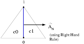
Ansys Fluent assigns adjacent cells to an interior face (c0 and
c1) according to the following convention: the cell
out of which a face area normal is pointing is designated as cell
C0, while the cell in to which a face area
normal is pointing is cell c1 (Figure 3.1: Ansys Fluent Determination of Face Area Normal Direction: 2D Face). In other words, face area normals always
point from cell c0 to cell c1.
The macros listed in Table 3.24: Macros for Boundary Face Flow Variables Defined in mem.h access flow variables at a boundary face.
Note: For boundaries with the density-based solver, note the following:
Enthalpy (
F_H(f,t)) is not stored.The boundary velocity array (
F_U(f,t),F_V(f,t), andF_W(f,t)) is not allocated for boundaries of type wall, symmetry, or axis.It is recommended that you use the
NNULLP()macro to avoid reading unallocated memory. For example, memory storage for the x-velocity variable can be checked by the following:/* check for x-velocity boundary storage */ if(NNULLP(THREAD_STORAGE(t, SV_U))) { … }
Table 3.24: Macros for Boundary Face Flow Variables Defined in mem.h
|
Macro |
Argument Types |
Returns |
|---|---|---|
|
|
|
u velocity |
|
|
|
v velocity |
|
|
|
w velocity |
|
|
|
temperature |
|
|
|
enthalpy |
|
|
|
turbulent kinetic energy |
|
|
|
turbulent kinetic energy dissipation rate |
|
|
|
species mass fraction |
See
DEFINE_UDS_FLUX
for an example UDF that utilizes
some of these macros.
The macros listed in Table 3.25: Macros for Interior and Boundary Face Flow Variables Defined in mem.h access flow variables at interior faces and boundary faces.
Table 3.25: Macros for Interior and Boundary Face Flow Variables Defined in mem.h
|
Macro |
Argument Types |
Returns |
|---|---|---|
|
|
|
pressure |
|
|
|
mass flow rate through a face |
F_FLUX can be used to return the
real scalar mass flow rate through a given face
f in a face thread t. The sign of
F_FLUX that is computed by the Ansys Fluent solver is positive if the
flow direction is the same as the face area normal direction (as determined by
F_AREA - see Face Area Vector (F_AREA)), and is
negative if the flow direction and the face area normal directions are opposite. In other
words, the flux is positive if the flow is out of the domain, and is
negative if the flow is in to the domain.
Note that the sign of the flux that is computed by the solver is opposite to that which is reported in the Ansys Fluent GUI (for example, the Flux Reports dialog box).
Important: F_P(f,t) is not available in the density-based
solver.
In the density-based solver, F_FLUX(f,t) will only return a
value if one or more scalar equations (for example, turbulence quantities) are being
solved that require the mass flux of a face to be stored by the solver.
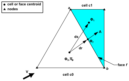
Ansys Fluent provides macros that allow the vectors connecting cell centroids and the vectors connecting cell and face centroids to be readily defined. These macros return information that is helpful in evaluating face values of scalars which are generally not stored, as well as the diffusive flux of scalars across cell boundaries. The geometry and gradients involved with these macros are summarized in Figure 3.2: Adjacent Cells c0 and c1 with Vector and Gradient Definitions.
To better understand the parameters that are returned by these macros, it is best to
consider how the aforementioned calculations are evaluated. Assuming that the gradient of a
scalar is available, the face value of a scalar,  , can be approximated by
 | (3–1) |
where  is the vector that connects the cell centroid with the face centroid. The
gradient in this case is evaluated at the cell centroid where
is the vector that connects the cell centroid with the face centroid. The
gradient in this case is evaluated at the cell centroid where  is also stored.
The diffusive flux,  , across a face,
  , of a scalar
  is given by,
 | (3–2) |
where  is the diffusion coefficient at the face. In Ansys Fluent’s
unstructured solver, the gradient along the face normal direction may be approximated by
evaluating gradients along the directions that connect cell centroids and along a direction
confined within the plane of the face. Given this,
is the diffusion coefficient at the face. In Ansys Fluent’s
unstructured solver, the gradient along the face normal direction may be approximated by
evaluating gradients along the directions that connect cell centroids and along a direction
confined within the plane of the face. Given this,  maybe approximated as,
 | (3–3) |
where the first term on the right hand side represents the primary gradient directed
along the vector  and the second term represents the ‘cross’ diffusion term.
In this equation,
and the second term represents the ‘cross’ diffusion term.
In this equation,  is the area normal vector of face
  directed from cell
 c0 to
c1,  is the distance between the cell centroids, and
  is the unit normal vector in this direction.
  is the average of the gradients at the two adjacent cells. (For boundary
faces, the variable is the gradient of the c0 cell.) This is shown in Figure 3.2: Adjacent Cells c0 and c1 with Vector and Gradient Definitions.
is the average of the gradients at the two adjacent cells. (For boundary
faces, the variable is the gradient of the c0 cell.) This is shown in Figure 3.2: Adjacent Cells c0 and c1 with Vector and Gradient Definitions.
The cells on either side of a face may or may not belong to the same cell thread.
Referring to Figure 3.2: Adjacent Cells c0 and c1 with Vector and Gradient Definitions, if a face is on the
boundary of a domain, then only c0 exists.
(c1 is undefined for an external face). Alternatively, if the
face is in the interior of the domain, then both c0 and
c1 exist.
There are two macros, F_C0(f,t) and
F_C1(f,t), that can be used to identify cells that are adjacent
to a given face thread t. F_C0 expands
to a function that returns the index of a face’s neighboring
c0 cell (Figure 3.2: Adjacent Cells c0 and c1 with Vector and Gradient Definitions),
while F_C1 returns the cell index for c1
(Figure 3.2: Adjacent Cells c0 and c1 with Vector and Gradient Definitions), if it exists.
Table 3.26: Adjacent Cell Index Macros Defined in mem.h
|
Macro |
Argument Types |
Returns |
|---|---|---|
|
|
|
|
|
|
|
|
See
DEFINE_UDS_FLUX
for an example UDF that utilizes
F_C0.
The cells on either side of a face may or may not belong to the same cell thread.
Referring to Figure 3.2: Adjacent Cells c0 and c1 with Vector and Gradient Definitions, if a face is on the
boundary of a domain, then only c0 exists.
(c1 is undefined for an external face). Alternatively, if the
face is in the interior of the domain, then both c0 and
c1 exist.
There are two macros, THREAD_T0(t) and
THREAD_T1(t), that can be used to identify cell threads that
are adjacent to a given face f in a face thread
t. THREAD_T0 expands to a function
that returns the cell thread of a given face’s adjacent cell
c0, and THREAD_T1 returns the cell
thread for c1 (if it exists).
Table 3.27: Adjacent Cell Thread Macros Defined in mem.h
|
Macro |
Argument Types |
Returns |
|---|---|---|
|
|
|
cell thread pointer for cell c0 |
|
|
|
cell thread pointer for cell c1 |
INTERIOR_FACE_GEOMETRY(f,t,A,ds,es,A_by_es,dr0,dr1) expands to a
function that outputs the following variables to the solver, for a given face
f, on face thread t. The macro is
defined in the sg.h header file which is not
included in udf.h. You will need to include this file in your UDF
using the #include directive.
|
|
the area normal vector |
|
|
distance between the cell centroids |
|
|
the unit normal vector in the direction from cell c0 to c1 |
|
|
the value |
|
|
vector that connects the centroid of cell |
|
|
the vector that connects the centroid of cell |

Note that INTERIOR_FACE_GEOMETRY can be called to retrieve
some of the terms needed to evaluate Equation 3–1 and Equation 3–3.
BOUNDARY_FACE_GEOMETRY(f,t,A,ds,es,A_by_es,dr0) expands to a
function that outputs the following variables to the solver, for a given face
f, on face thread t. It is defined in
the sg.h header file which is not included in
udf.h. You will need to include this file in your UDF using the
#include directive.
BOUNDARY_FACE_GEOMETRY can be called to retrieve some of the
terms needed to evaluate Equation 3–1 and Equation 3–3.
|
|
area normal vector |
|
|
distance between the cell centroid and the face centroid |
|
|
unit normal vector in the direction from centroid of cell c0 to the face centroid |
|
|
value |
|
|
vector that connects the centroid of cell |

BOUNDARY_FACE_THREAD_P(t) expands to a function that returns
TRUE if Thread *t is a boundary face
thread. The macro is defined in threads.h which is included in
udf.h. See
DEFINE_UDS_FLUX
for an
example UDF that utilizes BOUNDARY_FACE_THREAD_P.
BOUNDARY_SECONDARY_GRADIENT_SOURCE(source,n,dphi,dx,A_by_es,k)
expands to a function that outputs the following variables to the solver, for a given face
and face thread. It is defined in the sg.h header file which is
not included in udf.h. You will need to
include this file in your UDF using the #include
directive.
Important: The use of BOUNDARY_SECONDARY_GRADIENT_SOURCE first
requires that cell geometry information be defined, which can be readily obtained by the
use of the BOUNDARY_FACE_GEOMETRY macro (described previously
in this section). See Implementing Ansys Fluent’s P-1 Radiation Model Using User-Defined
Scalars for an
example.
BOUNDARY_SECONDARY_GRADIENT_SOURCE can be called to retrieve some
of the terms needed to evaluate Equation 3–3.
|
|
the cross diffusion term of the diffusive flux (that is, the second term on the right side of Equation 3–3) |
|
|
the |
|
|
a dummy scratch variable array that stores the facial gradient value during the computation |
|
|
the unit normal vector in the direction from centroid of cell c0 to the face centroid |
|
|
the value |
|
|
the diffusion coefficient at the face ( |


Important: Note that the gradient field variable addressed by the Svar
value n is not always allocated, and so your UDF must verify
its status (using the NULLP or NNULLP
function, as described in NULLP & NNULLP
) and assign a
value as necessary. See Implementing Ansys Fluent’s P-1 Radiation Model Using User-Defined
Scalars for an
example.
The macros listed in this section are special macros that are used often in UDFs.
Lookup_ThreadTHREAD_IDGet_DomainF_PROFILETHREAD_SHADOW
You can use Lookup_Thread when you want to retrieve the
pointer t to the thread that is associated with a given integer
zone ID number for a boundary zone. The zone_ID that is passed to
the macro is the zone number that Ansys Fluent assigns to the boundary and displays in the
boundary condition dialog box (for example, Fluid). Note that
this macro does the inverse of THREAD_ID (see below).
There are two arguments to Lookup_Thread.
domain is passed by Ansys Fluent and is the pointer to the domain
structure. You supply the integer value of zone_ID.
For example, the code
int zone_ID = 2; Thread *thread_name = Lookup_Thread(domain,zone_ID);
passes a zone ID of  to
to Lookup_Thread. A zone ID of  may, for example, correspond to a wall zone in your case.
Now suppose that your UDF needs to operate on a particular thread in a domain (instead
of looping over all threads), and the DEFINE macro you are using
to define your UDF does not have the thread pointer passed to it
from the solver (for example, DEFINE_ADJUST). You can use
Lookup_Thread in your UDF to get the desired thread pointer.
This is a two-step process.
First, you will need to get the integer ID of the zone by visiting the boundary
condition dialog box (for example, Fluid) and noting the zone ID. You
can also obtain the value of the Zone ID from the solver using
RP_Get_Integer. Note that in order to use
RP_Get_Integer, you will have to define the zone ID variable
first on the Scheme side using rp-var-define or
make-new-rpvar (see Scheme Macros for details.)
Next, you supply the zone_ID as an argument to
Lookup_Thread either as a hard-coded integer (for example,
1, 2) or as the variable assigned from
RP_Get_Integer. Lookup_Thread returns
the pointer to the thread that is associated with the given zone
ID. You can then assign the thread pointer to a thread_name and
use it in your UDF.
Important: Note that when Lookup_Thread is utilized in a multiphase
flow problem, the domain pointer that is passed to the function depends on the UDF that
it is contained within. For example, if Lookup_Thread is used
in an adjust function (DEFINE_ADJUST), then the mixture domain
is passed and the thread pointer returned is the mixture-level thread.
Example
Below is a UDF that uses Lookup_Thread. In this example, the
pointer to the thread for a given zone_ID is retrieved by
Lookup_Thread and is assigned to
thread. The thread pointer is then
used in begin_f_loop to loop over all faces in the given thread,
and in F_CENTROID to get the face centroid value.
/*******************************************************************
Example of an adjust UDF that uses Lookup_Thread.
Note that if this UDF is applied to a multiphase flow problem,
the thread that is returned is the mixture-level thread
********************************************************************/
#include "udf.h"
/* domain passed to Adjust function is mixture domain for multiphase*/
DEFINE_ADJUST(print_f_centroids, domain)
{
real FC[2];
face_t f;
int ID = 1;
/* Zone ID for wall-1 zone from Boundary Conditions task page */
Thread *thread = Lookup_Thread(domain, ID);
begin_f_loop(f, thread)
{
F_CENTROID(FC,f,thread);
printf("x-coord = %f y-coord = %f", FC[0], FC[1]);
}
end_f_loop(f,thread)
}
You can use THREAD_ID when you want to retrieve the integer
zone ID number (displayed in a boundary conditions dialog box such as
Fluid) that is associated with a given thread pointer
t. Note that this macro does the inverse of
Lookup_Thread (see above).
int zone_ID = THREAD_ID(t);
You can use the Get_Domain macro to retrieve a domain pointer
when it is not explicitly passed as an argument to your UDF. This is commonly used in
ON_DEMAND functions since
DEFINE_ON_DEMAND is not passed any arguments from the Ansys Fluent
solver. It is also used in initialization and adjust functions for multiphase applications
where a phase domain pointer is needed but only a mixture pointer is passed.
Get_Domain(domain_id);
domain_id is an integer whose value is
1 for the mixture domain, but the values for the phase domains
can be any integer greater than 1. The ID for a particular phase
can be found be selecting it in the Phases dialog box in
Ansys Fluent.
![]() Setup → Models
→ Multiphase → Phases
Setup → Models
→ Multiphase → Phases
![]() Edit...
Edit...
Single-Phase Flows
In the case of single-phase flows, domain_id is
1 and Get_Domain(1) will return the
fluid domain pointer.
DEFINE_ON_DEMAND(my_udf)
{
Domain *domain; /* domain is declared as a variable */
domain = Get_Domain(1); /* returns fluid domain pointer */
...
} Multiphase Flows
In the case of multiphase flows, the value returned by
Get_Domain is either the mixture-level, a phase-level, or an
interaction phase-level domain pointer. The value of domain_id is
always 1 for the mixture domain. You can obtain the
domain_id using the Ansys Fluent graphical user interface much in
the same way that you can determine the zone ID from the Boundary
Conditions task page. Simply go to the Phases dialog box
in Ansys Fluent and select the desired phase. The domain_id will then
be displayed. You will need to hard code this integer ID as an argument to the macro as
shown below.
DEFINE_ON_DEMAND(my_udf)
{
Domain *mixture_domain;
mixture_domain = Get_Domain(1); /* returns mixture domain pointer */
/* and assigns to variable */
Domain *subdomain;
subdomain = Get_Domain(2); /* returns phase with ID=2 domain pointer*/
/* and assigns to variable */
...
} Example
The following example is a UDF named get_coords that prints
the thread face centroids for two specified thread IDs. The function implements the
Get_Domain utility for a single-phase application. In this
example, the function Print_Thread_Face_Centroids uses the
Lookup_Thread function to determine the pointer to a thread,
and then writes the face centroids of all the faces in a specified thread to a file. The
Get_Domain(1) function call returns the pointer to the domain
(or mixture domain, in the case of a multiphase application). This argument is not passed
to DEFINE_ON_DEMAND.
/*****************************************************************
Example of UDF for single phase that uses Get_Domain utility
******************************************************************/
#include "udf.h"
FILE *fout;
void Print_Thread_Face_Centroids(Domain *domain, int id)
{
real FC[3];
face_t f;
Thread *t = Lookup_Thread(domain, id);
fprintf(fout,"thread id %d\n", id);
begin_f_loop(f,t)
{
F_CENTROID(FC,f,t);
fprintf(fout, "f%d %g %g %g\n", f, FC[0], FC[1], FC[2]);
}
end_f_loop(f,t)
fprintf(fout, "\n");
}
DEFINE_ON_DEMAND(get_coords)
{
Domain *domain;
domain = Get_Domain(1);
fout = fopen("faces.out", "w");
Print_Thread_Face_Centroids(domain, 2);
Print_Thread_Face_Centroids(domain, 4);
fclose(fout);
}
Note that Get_Domain(1) replaces the extern
Domain *domain expression used in releases of Ansys Fluent
6.
F_PROFILE is typically used in a
DEFINE_PROFILE UDF to set a boundary condition value in memory
for a given face and thread. The index i that is an argument to
F_PROFILE is also an argument to
DEFINE_PROFILE and identifies the particular boundary variable
(for example, pressure, temperature, velocity) that is to be set.
F_PROFILE is defined in mem.h.
|
Macro: |
|
|
Argument types: |
|
|
Function returns: |
|
The arguments of F_PROFILE are f,
the index of the face face_t; t, a
pointer to the face’s thread t; and
i, an integer index to the particular face variable that is to
be set. i is defined by Ansys Fluent when you hook a
DEFINE_PROFILE UDF to a particular variable (for example,
pressure, temperature, velocity) in a boundary condition dialog box. This index is passed
to your UDF by the Ansys Fluent solver so that the function knows which variable to operate
on.
Suppose you want to define a custom inlet boundary pressure profile for your Ansys Fluent case defined by the following equation:

You can set the pressure profile using a DEFINE_PROFILE UDF.
Since a profile is an array of data, your UDF will need to create the pressure array by
looping over all faces in the boundary zone, and for each face, set the pressure value
using F_PROFILE. In the sample UDF source code shown below, the
 coordinate of the centroid is obtained using
F_CENTROID, and this value is used in the pressure calculation
that is stored for each face. The solver passes the UDF the right index to the pressure
variable because the UDF is hooked to Gauge Total Pressure in the
Pressure Inlet boundary condition dialog box. See
DEFINE_PROFILE
for more information on
DEFINE_PROFILE UDFs.
/***********************************************************************
UDF for specifying a parabolic pressure profile boundary profile
************************************************************************/
#include "udf.h"
DEFINE_PROFILE(pressure_profile,t,i)
{
real x[ND_ND]; /* this will hold the position vector */
real y;
face_t f;
begin_f_loop(f,t)
{
F_CENTROID(x,f,t);
y = x[1];
F_PROFILE(f,t,i) = 1.1e5 - y*y/(.0745*.0745)*0.1e5;
}
end_f_loop(f,t)
}
THREAD_SHADOW returns the face thread that is the shadow of
Thread *t if it is one of a face/face-shadow pair that makes up
a thin wall. It returns NULL if the boundary is not part of a
thin wall and is often used in an if statement such as:
if (!NULLP(ts = THREAD_SHADOW(t)))
{
/* Do things here using the shadow wall thread (ts) */
}
In transient simulations, Ansys Fluent can collect time-sampled data for postprocessing of time-averaged mean and RMS values of many solution variables. In addition, resolved Reynolds stresses and some other correlation functions can be calculated.
To access the quantities that can be evaluated during postprocessing, the following macros can be used:
Mean Values
Pressure/Velocity Components:
P_mean=C_STORAGE_R(c,t, SV_P_MEAN)/delta_time_sampled;u_mean=C_STORAGE_R(c,t, SV_U_MEAN)/delta_time_sampled;v_mean=C_STORAGE_R(c,t, SV_V_MEAN)/delta_time_sampled;w_mean=C_STORAGE_R(c,t, SV_W_MEAN)/delta_time_sampled;Temperature/Species Mass Fraction:
T_mean=C_STORAGE_R(c,t, SV_T_MEAN)/delta_time_sampled;YI_mean=C_STORAGE_R_XV(c,t, SV_Y_MEAN,n)/delta_time_sampled_species[n];Mixture Fraction/Progress Variable:
Mixture_mean=C_STORAGE_R(c,t, SV_F_MEAN)/delta_time_sampled_non_premix;progress_mean=C_STORAGE_R(c,t, SV_C_MEAN)/delta_time_sampled_premix;
These quantities, as well as many others, may or may not be available depending on what models have been activated. Access to all of them always follows the same structure.
Note: The storage variable identifiers
SV_..._MEANdo not refer directly to time-averaged quantities. Instead, these storage variables contain the time-integral of these variables. It is necessary to divide by the sampling time to obtain the time averaged values.RMS Values
Pressure/Velocity Components:
P_rms=RMS(C_STORAGE_R(c,t, SV_P_MEAN), C_STORAGE_R(c,t, SV_P_RMS), delta_time_sampled, SQR(delta_time_sampled));u_rms=RMS(C_STORAGE_R(c,t, SV_U_MEAN), C_STORAGE_R(c,t, SV_U_RMS), delta_time_sampled, SQR(delta_time_sampled));v_rms=RMS(C_STORAGE_R(c,t, SV_V_MEAN), C_STORAGE_R(c,t, SV_V_RMS), delta_time_sampled, SQR(delta_time_sampled));w_rms=RMS(C_STORAGE_R(c,t, SV_W_MEAN), C_STORAGE_R(c,t, SV_W_RMS), delta_time_sampled, SQR(delta_time_sampled));Temperature/Species Mass Fraction:
T_rms=RMS(C_STORAGE_R(c,t, SV_T_MEAN), C_STORAGE_R(c,t, SV_T_RMS), delta_time_sampled, SQR(delta_time_sampled));YI_rms=RMS(C_STORAGE_R(c,t, SV_YI_MEAN(n)), C_STORAGE_R(c,t, SV_YI_RMS(n)), delta_time_sampled_species[n], SQR(delta_time_sampled));
The
RMSpreprocessor macro must be defined before it is used:#define RMS(mean_accum, rms_accum, n, nsq) \ sqrt(fabs(rms_accum/n - SQR(mean_accum)/nsq))
Again, these quantities, as well as many others, may or may not be available depending on what models have been activated. Access to all of them always follows the same structure.
Note: The storage variable identifiers
SV_..._RMScontain the time-integral of the square of the solution variables. It is necessary to divide by the sampling time to obtain the time averaged values.Resolved Reynolds (Shear) Stresses
UV:
uiuj =
CROSS_CORRELATION(C_STORAGE_R(c,t, SV_U_MEAN), C_STORAGE_R(c,t, SV_V_MEAN), C_STORAGE_R(c,t, SV_UV_MEAN), delta_time_sampled_shear, SQR(delta_time_sampled));UW:
uiuj =
CROSS_CORRELATION(C_STORAGE_R(c,t, SV_U_MEAN), C_STORAGE_R(c,t, SV_W_MEAN), C_STORAGE_R(c,t, SV_UW_MEAN), delta_time_sampled_shear, SQR(delta_time_sampled));VW:
uiuj =
CROSS_CORRELATION(C_STORAGE_R(c,t, SV_V_MEAN), C_STORAGE_R(c,t, SV_W_MEAN), C_STORAGE_R(c,t, SV_VW_MEAN), delta_time_sampled_shear, SQR(delta_time_sampled));As before, the
CROSS_CORRELATIONpreprocessor macro must be defined before it is used:#define CROSS_CORRELATION(mean_accum_1, mean_accum_2, cross_accum, n_cross, nsq_mean) \ (cross_accum/n_cross - (mean_accum_1*mean_accum_2)/nsq_mean)
These quantities, as well as many others, may or may not be available depending on what models have been activated. Access to all of them always follows the same structure.
Note: The
SV_UV/UW/VW_MEANstorage variables contain time-integrals of the products of two different storage variables each. In addition to the Reynolds stresses,SV_[U|V|W]T_MEANare available to calculate temperature-velocity component correlations as shown below:ut =
CROSS_CORRELATION(C_STORAGE_R(c,t, SV_U_MEAN), C_STORAGE_R(c,t, SV_T_MEAN), C_STORAGE_R(c,t, SV_UT_MEAN), delta_time_sampled_heat_flux, SQR(delta_time_sampled));
The macros listed in Table 3.28: Macros for Particles at Current Position Defined in
dpm_types.h
– Table 3.33: Macros for Particle Material Properties Defined in dpm_laws.h
can be used to return real
variables associated with the Discrete Phase Model (DPM), in SI units (where relevant).
They are typically used in DPM UDFs that are described in Discrete Phase Model (DPM) DEFINE Macros. The variables are available in both the pressure-based
and the density-based solvers. The macros are defined in the
dpm_types.h and dpm_laws.h header files, which
are included in udf.h.
The variable tp indicates a pointer to the
Tracked_Particle structure (Tracked_Particle
*tp) which gives you the value for the particle at the current position,
the variable m indicates a pointer to the relevant Material
structure (Material *m), and the real variable t is the
temperature.
Refer to the following sections for examples of UDFs that use some of these macros:
DEFINE_DPM_LAW
,
DEFINE_DPM_BC
,
DEFINE_DPM_INJECTION_INIT
,
DEFINE_DPM_SWITCH
, and
DEFINE_DPM_PROPERTY
.
The TP_... macros listed in Table 3.28: Macros for Particles at Current Position Defined in
dpm_types.h
through Table 3.32: Macros for Particle Species, Laws, Materials, and User Scalars Defined in
dpm_types.h
are to be used to access elements of
variables of the type Tracked_Particles or elements within
instances of the data structure pointed to by pointer variables of the type
Tracked_Particle *.
In addition, the dpm_types.h header file also contains
definitions for the PP_... macros that are analogous to the
corresponding TP_... macros. The PP_...
macros are similar in function, but they are to be used for accessing elements of
variables of the Particle or elements within the data structure
that are pointed to by pointer variables of the type Particle *.
Important: The TP_.... and analogous PP_...
macros should not be used interchangeably. Their definitions may be modified without
notice in future releases.
Table 3.28: Macros for Particles at Current Position Defined in dpm_types.h
|
Macro |
Argument Types |
Returns |
|---|---|---|
|
|
|
position |
|
|
|
velocity |
|
|
|
diameter |
|
|
|
temperature |
|
|
|
density |
|
|
|
mass |
|
|
|
current particle time |
|
|
|
time step |
|
|
|
flow rate of particles in a stream in kg/s (see below for details) |
|
|
|
liquid mass fraction (wet combusting particles only) |
|
|
|
liquid volume fraction (wet combusting particles only) |
|
|
|
volatile fraction (combusting particles only) |
|
|
|
char mass fraction (combusting particles only) |
|
|
|
volatile fraction remaining (two competing rates devolatilization model only) |
TP_FLOW_RATE(tp)
Each particle in a steady flow calculation represents a "stream" of many particles
that follow the same path. The number of particles in this stream that passes a particular
point in a second is the "strength" of the stream.
TP_FLOW_RATE(tp) returns the strength multiplied by
TP_INIT_MASS(tp) at the current particle position.
Table 3.29: Macros for Particles at Entry to Current Cell Defined in dpm_types.h
|
Macro |
Argument Types |
Returns |
|---|---|---|
|
|
|
position |
|
|
|
velocity |
|
|
|
diameter |
|
|
|
temperature |
|
|
|
density |
|
|
|
mass |
|
|
|
particle time at entry |
|
|
|
liquid mass fraction (wet combusting particles only) |
Important: Note that when you are using the macros listed in Table 3.29: Macros for Particles at Entry to Current Cell Defined in dpm_types.h to track transient particles, the particle state is the beginning of the fluid flow time step only if the particle does not cross a cell boundary.
Table 3.30: Macros for Particle Cell Index and Thread Pointer Defined in dpm_types.h
|
Name (Arguments) |
Argument Types |
Returns |
|---|---|---|
|
|
|
|
|
|
|
Thread |
|
|
|
The address of the variable |
|
|
|
|
|
|
|
Thread |
Table 3.31: Macros for Particles at Injection into Domain Defined in dpm_types.h
|
Macro |
Argument Types |
Returns |
|---|---|---|
|
|
|
position |
|
|
|
velocity |
|
|
|
diameter |
|
|
|
temperature |
|
|
|
density |
|
|
|
mass |
|
|
|
liquid mass fraction (wet combusting particles only) |
Table 3.32: Macros for Particle Species, Laws, Materials, and User Scalars Defined in dpm_types.h
|
Macro |
Argument Types |
Returns |
|---|---|---|
|
|
|
evaporating species index in mixture |
|
|
|
devolatilizing species index in mixture |
|
|
|
oxidizing species index in mixture |
|
|
|
combustion products species index in mixture |
|
|
|
int law, current particle law index |
|
|
|
int next_law, next particle law index |
|
|
|
Material *m, material pointer |
|
|
|
storage array for user-defined values (indexed by
|
Table 3.33: Macros for Particle Material Properties Defined in dpm_laws.h
|
Macro |
Argument Types |
Returns |
|---|---|---|
|
|
|
boiling temperature |
|
|
|
Binary diffusion coefficient to be used in the gaseous boundary layer around the particle |
|
|
|
emissivity and scattering factor for the radiation model |
|
|
|
thermal conductivity |
|
|
|
heat of pyrolysis |
|
|
|
heat of reaction |
|
|
|
latent heat |
|
|
|
specific heat of material used for liquid associated with particle |
|
|
|
dynamic viscosity of liquid part of particle |
|
|
|
particle density |
|
|
|
specific heat |
|
|
|
swelling coefficient for devolatilization |
|
|
|
surface tension of liquid part of particles |
|
|
|
vapor pressure of liquid part of particle |
|
|
|
vaporization temperature used to switch to vaporization law |
Table 3.34: Macros to access source terms on CFD cells for the DPM model
|
Macro |
Argument Types |
Returns |
|---|---|---|
|
|
|
momentum source (SI units: kg m/s2), explicit |
|
|
|
momentum source (SI units: kg/s), implicit |
|
|
|
momentum source swirl component (SI units: kg m/s2), explicit |
|
|
|
momentum source swirl component (SI units: kg/s), implicit |
|
|
|
energy source (SI units: J/s), explicit |
|
|
|
energy source (SI units: J/K/s), implicit |
|
|
|
species mass source (SI units: kg/s), explicit |
|
|
|
species mass source (SI units: kg/s), implicit |
|
|
|
reaction rates of particle REACTIONS (SI units: kg/s/m3) |
|
|
|
vaporization mass source of material |
|
|
|
devolatilization mass source of material |
|
|
|
burnout mass source of material |
|
|
|
mass source of pdf stream 1 (SI units: kg/s) |
|
|
|
mass source of pdf stream 2 (SI units: kg/s) |
|
|
|
particles emissivity (SI units: m2K4) |
|
|
|
particles absorption coefficient (SI units: m3/m) |
|
|
|
particles scattering coefficient (SI units: m3/m) |
|
|
|
burnout mass source (SI units: kg/s) |
|
|
|
concentration of particles (SI units: kg/m3) |
|
|
|
concentration of particle surface species (SI units: kg/m3) |
Note:
The macros listed in Table 3.34: Macros to access source terms on CFD cells for the DPM model in general are not intended to be used to assign values inside
DEFINE_DPM_SOURCE.By design, you cannot assign values to some macros, such as
C_DPMS_YIandC_DPMS_YI_AP. These macros are used only for reporting purposes inDEFINE_ADJUSTandDEFINE_ON_DEMAND.
The following macros can be used in NOx model UDFs in the calculation of pollutant
rates. These macros are defined in the header file sg_nox.h, which is
included in udf.h. They can be used to return
real NOx variables in SI units, and are available in both the
pressure-based and the density-based solvers. See
DEFINE_NOX_RATE
for examples of
DEFINE_NOX_RATE UDFs that use these macros.
Table 3.35: Macros for NOx UDFs Defined in sg_nox.h
|
Macro |
Returns |
|---|---|
|
|
index of pollutant equation being solved (see below) |
|
|
molar concentration of species specified by |
|
|
TRUE if the species specified by |
|
|
Arrhenius rate calculated from the constants specified by
|
|
|
production rate of the pollutant species being solved |
|
|
reduction rate of the pollutant species being solved |
|
|
quasi-steady rate of N2O formation (if the quasi-steady model is used) |
|
|
fluctuating density value (or, if no PDF model is used, mean density at a given cell |
|
|
fluctuating temperature value (or, if no PDF model is used, mean temperature at a given cell) |
|
|
fluctuating mass fraction value (or, if no PDF model is used, mean mass
fraction at a given cell) of the species given by index
|
|
|
upper limit for the temperature PDF integration (see below) |
Important:
Pollut_Par is a pointer to the
Pollut_Parameter data structure that contains auxiliary data
common to all pollutant species and NOx is a pointer to the
NOx_Parameter data structure that contains data specific to
the NOx model.
POLLUT_EQN(Pollut_Par)returns the index of the pollutant equation currently being solved. The indices areEQ_NOfor NO,EQ_HCNfor HCN,EQ_N2Ofor O, and
 EQ_NH3for .
.MOLECON(Pollut,SPE)returns the molar concentration of a species specified bySPE, which is either the name of the species orIDX(i)when the species is a pollutant (like NO).SPEmust be replaced by one of the following identifiers:FUEL, O2, O, OH, H2O, N2, N, CH, CH2, CH3, IDX(NO), IDX(N2O), IDX(HCN), IDX(NH3). For example, for molar concentration you should call
 MOLECON(Pollut, O2), whereas for NO molar concentration the call should beMOLECON(Pollut, IDX(NO)). The identifierFUELrepresents the fuel species as specified in the Fuel Species drop-down list under Prompt NO Parameters in the NOx Model dialog box.ARRH(Pollut,K)returns the Arrhenius rate calculated from the constants specified byK.Kis defined using theRate_Constdata type and has three elements - A, B, and C. The Arrhenius rate is given in the form of
where T is the temperature.
Note that the units of
Kmust be in m-mol-J-s.POLLUT_CTMAX(Pollut_Par)can be used to modify the value used as the upper limit for the integration of the temperature
PDF (when temperature is accounted for in the turbulence interaction modeling). You
must make sure not to put this macro under any conditions within the UDF (for example,
value used as the upper limit for the integration of the temperature
PDF (when temperature is accounted for in the turbulence interaction modeling). You
must make sure not to put this macro under any conditions within the UDF (for example,
IN_PDForOUT_PDF).
The macros listed in Table 3.36: Macros for Dynamic Mesh Variables Defined in dynamesh_tools.h
are useful in dynamic
mesh UDFs. The argument dt is a pointer to the dynamic thread
structure, and time is a real value. These macros are defined in
the dynamesh_tools.h.
Table 3.36: Macros for Dynamic Mesh Variables Defined in dynamesh_tools.h
|
Name (Arguments) |
Argument Types |
Returns |
|---|---|---|
|
|
|
pointer to a thread |
|
|
|
center of gravity vector |
|
|
|
cg velocity vector |
|
|
|
angular velocity vector |
|
|
|
orientation of body-fixed axis vector |
|
|
N/A |
current dynamic mesh time |
|
|
|
absolute value of the crank angle |
See
DEFINE_GRID_MOTION
for an example UDF that utilizes
DT_THREAD.
The macros listed in Table 3.37: Macros for Battery UDFs Defined in sg_mem.h can be used in a UDF to access the MSMD battery model variables. These macros are defined in the header file sg_mem.h, which is included in udf.h. They can be used to return real variables in SI units. Note that they are available only if the MSMD solution method is used in a simulation.
Table 3.37: Macros for Battery UDFs Defined in sg_mem.h
|
Macro |
Returns |
|---|---|
|
|
degree of discharge (-) |
|
|
volumetric contact resistance in the internal short circuit model (ohm m3) |
|
|
heat source due to Joule heating (W/m3) |
|
|
heat source due to electrochemical reaction (W/m3) |
|
|
heat source due to internal short (W/m3) |
|
|
heat source due to thermal abuse reactions (W/m3) |
|
|
total heat source (W/m3) |
|
|
reaction progress variable for the decomposition reaction of SEI layer (-) in the four-equation thermal abuse model |
|
|
reaction progress variable for the decomposition reaction between positive
electrode and solvent (-) in the four-equation thermal abuse model, or the
reaction progress variable |
|
|
reaction progress variable for the decomposition reaction between negative electrode and solvent (-) in the four-equation thermal abuse model |
|
|
reaction progress variable for the decomposition reaction of electrolyte (-) in the four-equation thermal abuse model |
|
|
reaction progress variable for the decomposition reaction due to internal short circuit (-) |
|
|
electric current component in x-direction (A/m2) |
|
|
electric current component in y-direction (A/m2) |
|
|
electric current component in z-direction (A/m2) |

You can create saturation tables for pure fluids, binary, and multi-species mixtures. Fluent provides the following functions that you can use in UDFs to compute saturation properties for the bubble and dew points for a single species or multiple-species:
When using a single-species NIST real gas model, Fluent provides a function that you can use in your UDFs to obtain saturation properties for the bubble and dew points. You can specify either temperature or pressure and the function will return an array containing the pressures or temperatures, respectively, and the liquid and vapor phase densities.
void getsatvalues_NIST(int index, double x, double y[]);
| where: | |
index = 0 if
x is a specified temperature | |
=
1 if x is a specified
pressure | |
x = temperature or pressure (according to value of
index) at which to obtain saturation properties | |
y[] = array of saturation properties |
The values returned in y[] depend on the choice of
index.
| Array elements |
index=0
|
index=1
| |
|---|---|---|---|
| Bubble Point |
y[0]
| pressure (Pa) | temperature (K) |
y[1]
| density of liquid (kg/m3) | density of liquid (kg/m3) | |
| Dew Point |
y[2]
| pressure (Pa) | temperature (K) |
y[3]
| density of vapor (kg/m3) | density of vapor (kg/m3) |
This function can be used regardless of whether you have enabled the lookup table.
int getsatvalues_NIST_msp (int index, double x, double y[], int
ibubbleordew)
This function is similar to the single-species function,
getsatvalues_NIST, but it applies to multi-species. For a given
temperature or pressure you can obtain the corresponding pressure or temperature and the
liquid and vapor phase densities.
In the function, index, x, and
ibubbleordew are inputs. If the
index=0, the input for x is
temperature and if the index=1, the input for
x is pressure. If ibubbleordew=0,
Fluent returns bubble point properties, otherwise it returns dew point properties.
y[] is an array of saturation properties.
The function returns an integer indicating the number of interpolation points for a given temperature and pressure:
0—no interpolation points, which could indicate that the given temperature and pressure is outside of the saturation curve range.
1—interpolation point with a bubble or dew curve.
2—interpolation points in the retrograde region of the saturation curves.
When index = 0:
| Bubble Point | Dew Point | |
|---|---|---|
| Function Returns 1 | ||
y[0] | Pressure | Pressure |
y[1] | Density (liquid) | Density (vapor) |
| Function Returns 2 | ||
y[0] | Pressure | Pressure |
y[1] | Density (liquid) | Density (vapor) |
y[2] | Pressure | Pressure |
y[3] | Density (liquid) | Density (vapor) |
When index = 1:
| Bubble Point | Dew Point | |
|---|---|---|
| Function Returns 1 | ||
y[0] | Temperature | Temperature |
y[1] | Density (liquid) | Density (vapor) |
| Function Returns 2 | ||
y[0] | Temperature | Temperature |
y[1] | Density (liquid) | Density (vapor) |
y[2] | Temperature | Temperature |
y[3] | Density (liquid) | Density (vapor) |
void get_satprop_NIST_msp (index, z, minrho, maxrho, nsat, npts, p_bub,
t_bub, p_dew, t_dew);
The 2nd function for multi-species can be used to generate a saturation table for variable compositions.
Inputs:
|
Argument |
Description |
|---|---|
|
|
0: composition in mass fractions >0: composition in mole fractions |
|
|
real array—composition of fluid (ensure sum=1) |
|
|
minimum density in moles per liter (0.1 is a reasonable default for most cases) |
|
|
maximum density in moles per liter (25 is a reasonable default for most cases) |
|
|
number of points in bubble/dew curves (minimum is 12) |
Outputs:
|
Argument |
Description |
|---|---|
|
|
actual number of bubble curve points returned by the function |
|
|
actual number of dew curve points returned by the function |
|
|
a pressure array of the bubble point curve returned by the function |
|
|
a temperature array of the bubble point curve returned by the function |
|
|
a pressure array of the dew point curve returned by the function |
|
|
a temperature array of the dew point curve returned by the function |
This function computes saturation data for the given composition in z. This could be a binary mixture, three species, or more.
To use get_satprop_NIST_msp in a UDF:
Start a Fluent session as normal.
Enter the text command
define/user-defined/real-gas-models/nist-multispecies-real-gas-modeland specify the number and species, but DO NOT activate the NIST-Table. This is only for generating user-defined bubble and dew point curves using NIST models.Ensure that the number and order of components selected in Fluent matches the number and order of species in
zof theget_satprop_NIST_mspfunction.Note: The output temperature and pressure arrays appear in ascending order for dew points and descending order for bubble points. However, when the output is for single-species, that is,
z[i]=1.0, allz[k]=0.0,(k=0,...,n; k!=i), they are in ascending order. The values for the critical condition are also presented in the output arrays. They are stored in the 1st element of the bubble point array and last element of the dew point array. For single-species, it is stored in the last element of the output arrays for both bubble and dew points.
This UDF, named getsat_msp, computes and writes saturation
curves. It demonstrates how a binary phase envelope is calculated using the NIST real
gas model.
#include "udf.h"
#include <string.h>
#define NUM_SAT 50
#define SMALL_NUM 1.e-6
DEFINE_ON_DEMAND(getsat_msp)
{
double t, p, y[10];
int np,index;
int nsat,npts[2];
double z[10]={0.}, minrho, maxrho;
double p_bub[NUM_SAT],t_bub[NUM_SAT],p_dew[NUM_SAT],t_dew[NUM_SAT];
FILE *fp1, *fp2;
int i,j,k,ncomps=2;
fp1 = fopen("NIST_Bub_Pnts_Curve.xy", "w");
fp2 = fopen("NIST_Dew_Pnts_Curve.xy", "w");
/* test on udf built NIST table - sat */
minrho = 0.1;
maxrho = 25.;
nsat = NUM_SAT;
z[0] = 0.;
fprintf(fp1, "(title \"Sat Bubble P-T\")");
fprintf(fp1, "\n(labels \"Temperature (K)\" \"Pressure (kPa)\")\n");
fprintf(fp2, "(title \"Sat Dew P-T\")");
fprintf(fp2, "\n(labels \"Temperature (K)\" \"Pressure (kPa)\")\n");
for (j=0; j<21; j++)
{
if (z[0] > 1.) z[0] = 1.;
z[1] = 1. - z[0];
if (z[1] < 0.) z[1] = 0.;
get_satprop_NIST_msp(0,z,minrho,maxrho,nsat,npts,p_bub,t_bub,p_dew,t_dew);
/* bubble */
for (i=0; i<1; i++)
fprintf(fp1, "\n((xy/key/label \"z[0]=%g numpts=%d\")\n",z[i],npts[0]);
if (fabs(z[0])<SMALL_NUM || fabs(z[0]-1.)<SMALL_NUM || fabs(z[1])<SMALL_NUM || fabs(z[1]-1.)<SMALL_NUM)
{
for (i=0;i<npts[0];i++)
fprintf(fp1, "%g\t %g\t \n",t_bub[i],p_bub[i]/1000.);
}
else
{
for (i=npts[0]-1;i>-1;i--)
fprintf(fp1, "%g\t %g\t \n",t_bub[i],p_bub[i]/1000.);
}
fprintf(fp1, ")\n");
/* dew */
for (i=0; i<1; i++)
fprintf(fp2, "\n((xy/key/label \"z[0]=%g numpts=%d\")\n",z[i],npts[1]);
for (i=0;i<npts[1];i++)
fprintf(fp2, "%g\t %g\t \n",t_dew[i],p_dew[i]/1000.);
fprintf(fp2, ")\n");
z[0] += 0.05;}
}
fclose(fp1);
fclose(fp2);
}
For given temperature, pressure, and mixture composition, you can obtain thermodynamic
properties of a mixture material in liquid, gas, and two-phase regimes using
get_prop_NIST_msp. NIST implements the GERG model for
thermodynamic properties of the mixtures. This model applies mixing rules to the Helmholtz
energy for each mixture components. Mixture data for the binary pairs can be found in
hmx.bnc provided with your Ansys Fluent installation.
Void get_prop_NIST_msp(double t, double p, double z[], double
prop[]);
|
Argument Type |
Description |
|---|---|
|
|
Temperature (K). |
|
|
Pressure (Pa). |
|
|
Real array, mass fractions of each component/species. The sum of the mass
fractions for all the materials in a mixture must be 1.
|
Function returns
double prop[]: Real array with thermodynamic properties as
follows.
|
Thermodynamic Properties Output | |
|---|---|
|
Vapor quality | |
|
|
vapor/gas moles/mixture moles
0<
|
|
|
vapor/gas mass fraction |
|
|
vapor/gas volume fraction |
|
Density (Kg/m^3) | |
|
|
bulk/mixture density |
|
|
liquid phase density |
|
|
vapor/gas phase density |
|
Specific-heat, cp (J/Kg-K) | |
|
|
bulk/mixture specific heat |
|
|
liquid phase specific heat |
|
|
vapor/gas phase specific heat |
|
Thermal conductivity (W/m-K) | |
|
|
bulk/mixture thermal conductivity |
|
|
liquid phase thermal conductivity |
|
|
vapor/gas phase thermal conductivity |
|
Viscosity (Pa-s) | |
|
|
bulk/mixture viscosity |
|
|
liquid phase viscosity |
|
|
vapor/gas phase viscosity |
|
Enthalpy (J/Kg) | |
|
|
bulk/mixture enthalpy |
|
|
liquid phase enthalpy |
|
|
vapor/gas phase enthalpy |
|
Speed of sound (m/s) | |
|
|
bulk speed of sound (0 if two-phase regime) |
|
|
in liquid phase |
|
|
in vapor/gas phase |
|
Component mass fractions in liquid phase | |
|
|
component/species, i = [0] … [n-1] |
|
Component mass fractions in vapor phase | |
|
|
component/species, i = [0] … [n-1] |
Important: The ranges of temperatures and pressures must be carefully selected, so that the limits on the material property application are not breached.
NIST is currently unable to calculate two-phase or mixture regime properties since all properties are relative to a pure or single phase. Ansys Fluent implements simple mixing rules based on volume fractions:

where  is the bulk property,
  refers to a liquid or vapor phase,
  are the phase specific properties in vapor and liquid, and
 is the volume fraction of the
  th phase.
You can embed the get_prop_NIST_msp UDF access macro in a
number of Fluent UDF functions, such as DEFINE_ON_DEMAND. For
example, you can use get_prop_NIST_msp to build a property
database with variables of temperature, pressure and composition.
To use the get_prop_NIST_msp access function, you must first
enable the NIST real gas model for multi-species by entering the following text command in
the Fluent console:
define/user-defined/real-gas-models/nist-multispecies-real-gas-model
use multispecies NIST real gas? [no]
yes
Once the model is enabled, the list of available pure-fluid materials that you can select will be displayed.
Then enter responses to the following prompts in the console:
Number of species [0]Enter the number of species that form the mixture.
select real-gas data file 1 []For each fluid material, enter the name enclosed in quotation marks. For example:
select real-gas data file 1 []"methane.fld"select real-gas data file 2 []"ethane.fld"Once the fluids are selected, Fluent prints a list of properties for each fluid material and its application ranges of temperature and pressure.
Create NIST LookUp Table for multi components?[no]Enter
noat the prompt.Follow the normal UDF practices.
If the input parameters for get_prop_NIST_msp are outside the
limits specified in NIST, the first element of the prop[] array,
prop[NIST_q_molar]=q, will return the value of
-2999.0. This indicates that NIST calculations of thermodynamic
properties are questionable or simply impossible for given temperature, pressure and/or
combination of materials. Since the returned value is a real double number, you can
capture this error by using an appropriate conditional statement, such as
if (q > -2999.1 && q < -2998.9)
The following UDF, named getprop_msp, is called from a
DEFINE_ON_DEMAND UDF Macro (
DEFINE_ON_DEMAND
). The function obtains thermodynamic properties
of a mixture consisting of seven species. The species names and mass fractions are
specified in the arrays spe_names[] and
spe_mfractions[], respectively. (Note that the
spe_mfractions[] array could also be variable.) The values of
these thermodynamic properties are generated by the NIST Real Gas Model (current Version
9.1) in Ansys Fluent. A series of temperature and pressure conditions are specified in the
arrays temp[] and press[],
respectively.
The obtained properties values are printed in the console and stored in the
NIST_output.txt file. Any errors messages are recorded in the
NIST_errors.txt file.
The UDF can be executed as an interpreted or compiled UDF in Ansys Fluent.
#include "udf.h"
#include <string.h>
#define NUM_MAX 150
#define SPE_MAX 20
#define N_SPE 7
#define N_DATA 6
DEFINE_ON_DEMAND(getprop_msp)
{
double t,p,q,sum;
double z[SPE_MAX]={0.};
FILE *fp1,*fp2;
int i,j,k,n,ncomps;
double prop[NUM_MAX]={0.};
double temp[N_DATA]={185,200,215,200,200,200};
double press[N_DATA]={5.e6,5.e6,5.e6,4.5e6,5.5e6,6.e6};
char *spe_names[N_SPE]={"methane","nitrogen","carbon-dioxide","ethane","propane","isobutane","butane"};
double spe_mfractions[N_SPE]={0.70061,0.20227,0.023246,0.053209,0.014306,0.0031167,0.0032414};
fp1 = fopen("NIST_output.txt","w");
fp2 = fopen("NIST_errors.txt","w");
/* testing nist property access function */
ncomps = N_SPE; /* number of species. to be matched by setting in fluent */
/* composition in mass fraction */
sum = 0.;
for (i=0; i<N_SPE; i++)
{
z[i] = spe_mfractions[i];
sum += z[i];
}
for (i=0; i<N_SPE; i++)
z[i] /= sum;
Message0("\nComposition (Mass Fractions): %d species\n",ncomps);
for (i=0; i<ncomps; i++)
Message0(" %s : %f ",spe_names[i],z[i]);
fprintf(fp1, "quality_molar, quality_mass, quality_vol, density, den_liq, den_vap, h, h_liq, h_vap,
cp, cp_liq, cp_vap, ktc, ktc_liq, ktc_vap, mu, mu_liq, mu_vap, ");
for (i=0; i<ncomps; i++)
fprintf(fp1, " %s_liq, ",spe_names[i]);
for (i=0; i<ncomps; i++)
fprintf(fp1, " %s_vap, ",spe_names[i]);
fprintf(fp1, " speed-of-sound");
fprintf(fp2, "NIST calculations questionable or not possible for the following given inputs\n");
fprintf(fp2, "\nPlease make sure the inputs are within permitted limits set by NIST!");
fprintf(fp2, "\nTemperature Pressure Composition: (Mass Fractions) ");
fprintf(fp2, "\n(K) (Pa) ");
for (i=0; i<ncomps; i++)
fprintf(fp2, " %s ",spe_names[i]);
for (k=0; k<N_DATA; k++)
{
t = temp[k];
p = press[k];
get_prop_NIST_msp(t,p,z,prop); /* call NIST property calculations */
q = prop[NIST_q_molar]; /* error handling */
if (q > -2999.1 && q < -2998.9)
{
fprintf(fp2, "\n%5.4e %5.4e ",t,p);
for (i=0; i<ncomps; i++)
fprintf(fp2, " %5.4e ",z[i]);
continue;
}
Message0("\n\ngetprop_msp: T=%f (K), P=%e (Bar) ",t,p/1.e5);
Message0("\n\nquality (mol/mol)=%f quality (kg/kg)=%f quality (vol/vol)=%f\n", prop[NIST_q_molar],
prop[NIST_q_mass],prop[NIST_q_vol]);
Message0("\n Bulk Liquid-Phase Vapor-Phase\n");
Message0("\ndensity (kg/m^3): %f %f %f\n",prop[NIST_den_m],
prop[NIST_den_l],prop[NIST_den_v]);
Message0("\nspecific-heat (kj/kg-k): %f %f %f\n",prop[NIST_cp_m]/1.e3,
prop[NIST_cp_l]/1.e3,prop[NIST_cp_v]/1.e3);
Message0("\nthermal-ktc (mk/m-k): %f %f %f\n",prop[NIST_ktc_m]*1.e3,
prop[NIST_ktc_l]*1.e3,prop[NIST_ktc_v]*1.e3);
Message0("\nviscosity (uPa-s): %f %f %f\n",prop[NIST_mu_m]*1.e6,
prop[NIST_mu_l]*1.e6,prop[NIST_mu_v]*1.e6);
Message0("\nenthalpy (kj/kg): %f %f %f\n",prop[NIST_h_m]/1.e3,
prop[NIST_h_l]/1.e3,prop[NIST_h_v]/1.e3);
Message0("\nspeed of sound (m/s): %f %f %f\n",prop[NIST_a_m],
prop[NIST_a_l],prop[NIST_a_v]);
Message0("\nMass fractions in liquid phase: ");
for (i=0; i<ncomps; i++)
Message0("%s : %f ",spe_names[i],prop[NIST_massfrac0_l+i]);
Message0("\nMass fractions in vapor phase: ");
for (i=0; i<ncomps; i++)
Message0("%s : %f ",spe_names[i],prop[NIST_massfrac0_v+i]);
/* quality */
fprintf(fp1, "\n%5.4f %5.4f %5.4f ", prop[NIST_q_molar],prop[NIST_q_mass],prop[NIST_q_vol]);
/* density (kg/m^3) */
fprintf(fp1, "%5.4f %5.4f %5.4f ",prop[NIST_den_m],prop[NIST_den_l],prop[NIST_den_v]);
/* enthalpy (KJ/Kg) */
fprintf(fp1, "%5.4f %5.4f %5.4f ",prop[NIST_h_m]/1.e3,prop[NIST_h_l]/1.e3,prop[NIST_h_v]/1.e3);
/* specific-heat cp (Kj/Kg-k) */
fprintf(fp1, "%5.4f %5.4f %5.4f ",prop[NIST_cp_m]/1.e3,prop[NIST_cp_l]/1.e3,prop[NIST_cp_v]/1.e3);
/* thermal conductivity (mw/m-k) */
fprintf(fp1, "%5.4f %5.4f %5.4f ",prop[NIST_ktc_m]*1.e3,prop[NIST_ktc_l]*1.e3,prop[NIST_ktc_v]*1.e3);
/* viscosity (uPa-s) */
fprintf(fp1, "%5.4f %5.4f %5.4f ",prop[NIST_mu_m]*1.e6,prop[NIST_mu_l]*1.e6,prop[NIST_mu_v]*1.e6);
/* Mass fractions in liquid phase */
for (i=0; i<ncomps; i++)
fprintf(fp1, "%5.4f ",prop[NIST_massfrac0_l+i]);
/* Mass fractions in vapor phase */
for (i=0; i<ncomps; i++)
fprintf(fp1, "%5.4f ",prop[NIST_massfrac0_v+i]);
/* speed of sound (m/s) */
fprintf(fp1, "%5.4f %5.4f %5.4f ",prop[NIST_a_m],prop[NIST_a_l],prop[NIST_a_v]);
}
fclose(fp1);
fclose(fp2);
}
This section contains macros that you can use when defining scalar transport UDFs in
Ansys Fluent. Note that if you try to use the macros listed below (for example,
F_UDSI, C_UDSI) before you have
specified user-defined scalars in your Ansys Fluent model (in the User-Defined
Scalars dialog box), then an error will result.
Ansys Fluent assigns a default name for every user-defined scalar that you allocate in the
graphical user-interface. For example, if you specify 2 as the
Number of User-Defined Scalars, then two variables with default
names User Scalar 0 and User Scalar 1
will be defined and the variables with these default names will appear in setup and
postprocessing dialog boxes. You can change the default names if you want, using
Set_User_Scalar_Name as described below.
The default name that appears in the graphical user interface and on plots in Ansys Fluent
for user-defined scalars (for example, User Scalar 0) can now be
changed using the function Set_User_Scalar_Name.
void Set_User_Scalar_Name(int i,char *name);
i is the index of the scalar and name is
a string containing the name you want to assign. It is defined in
sg_udms.h.
Set_User_Scalar_Name should be used only once and is best used in
an EXECUTE_ON_LOADING UDF (see
DEFINE_EXECUTE_ON_LOADING
). Due to the mechanism used, UDS
variables cannot be renamed after they have been set, so if the name is changed in a UDF,
for example, and the UDF library is reloaded, then the old name could remain. In this
case, restart Ansys Fluent and load the library again.
You can use F_UDSI when you want to access face variables
that are computed for user-defined scalar transport equations (Table 3.38: Accessing User-Defined Scalar Face Variables (mem.h)). See Example UDF that Utilizes UDM and UDS Variables for
an example of F_UDSI usage.
Table 3.38: Accessing User-Defined Scalar Face Variables (mem.h)
|
Macro |
Argument Types |
Returns |
|---|---|---|
|
|
Note: |
UDS face variables |
Important: Note that F_UDSI is available for wall and flow boundary
faces, only. If a UDS attempts to access any other face zone, then an error will
result.
You can use C_UDSI when you want to access cell variables
that are computed for user-defined scalar transport equations. Macros for accessing UDS
cell variables are listed in Table 3.39: C_UDSI for Accessing UDS Transport Cell Variables
(mem.h). Some examples of usage
for these macros include defining non-constant source terms for UDS transport equations
and initializing equations. See Example UDF that Utilizes UDM and UDS Variables for an
example of C_UDSI usage.
Table 3.39: C_UDSI for Accessing UDS Transport Cell Variables
(mem.h)
|
Macro |
Argument Types |
Returns |
|---|---|---|
|
|
|
UDS cell variables |
|
|
|
UDS gradient |
|
|
|
UDS previous time step |
|
|
|
UDS second previous time step |
|
|
Note: |
UDS diffusivity |
Note: The C_UDSI_M2(c,t,i) macro can only be used in a case that
is second order in time, that is, a case in which Second Order
Implicit or Bounded Second Order Implicit is selected
from the Transient Formulation drop-down list in the
Solution Methods task page.
Prior to use, you can reserve scalar variables to avoid data conflicts between
multiple UDF libraries using the same user-defined scalars (see Reserve_User_Scalar_Vars
).
The new capability of loading more than one UDF library into Ansys Fluent raises the
possibility of user-defined scalar (UDS) clashes. To avoid data contention between
multiple UDF libraries using the same user-defined scalars, Ansys Fluent has provided the
macro Reserve_User_Scalar_Vars that allows you to reserve scalars
prior to use.
int Reserve_User_Scalar_Vars(int num)
int num is the number of user-defined scalars that the library
uses. The integer returned is the lowest UDS index that the library may use. After
calling:
offset = Reserve_User_Scalar_Vars(int num);
the library may safely use C_UDSI(c,t,offset) to
C_UDSI(c,t,offset+num-1). See
DEFINE_EXECUTE_ON_LOADING
for an example of macro usage. Note
that there are other methods you can use within UDFs to hardcode the offset to prevent
data contention.
Reserve_User_Scalar_Vars (defined in
sg_udms.h) is designed to be called from an
EXECUTE_ON_LOADING UDF (
DEFINE_EXECUTE_ON_LOADING
). An on-loading UDF, as its name
implies, executes as soon as the shared library is loaded into Ansys Fluent. The macro can
also be called from an INIT or ON_DEMAND
UDF. After a user scalar has been reserved, it can be set to unique names for the
particular library using Set_User_Memory_Name (see below for
details on Set_User_Memory_Name). After the number of UDS that
are needed by a particular library is set in the GUI and the variables are successfully
reserved for the loaded library, the other functions in the library can safely use
C_UDMI(c,t,offset) up to
C_UDMI(c,t,offset+num-1) to store values in user scalars
without interference.
Ansys Fluent does not currently provide the capability to unreserve UDS variables using a
macro. Unreserve macros will be available in future versions of
Ansys Fluent.
This section contains macros that access user-defined memory (UDM) and user-defined node memory (UDNM) variables in Ansys Fluent.
Before you can store variables in memory using the macros provided below, you will first need to allocate the appropriate number of memory location(s) in the User-Defined Memory dialog box in Ansys Fluent.
![]() Parameters & Customization → User
Defined Memory
Parameters & Customization → User
Defined Memory ![]() Edit...
Edit...
Important: Note that if you try to use F_UDMI,
C_UDMI, or N_UDMI before you have
allocated memory, then an error will result.
A variable will be created for every user-defined memory and user-defined node memory
location that you allocate in the graphical user interface. For example, if you specify
2 as the Number of User-Defined Memory
Locations or Number of User-Defined Node Memory
Locations, then two variables with default names User Memory
0 and User Memory 1, or User Node Memory
0 and User Node Memory 1 will be defined for your
model and the default variable names will appear in postprocessing dialog boxes. You can
change the default names if you want, using Set_User_Memory_Name or
Set_User_Node_Memory_Name as described below.
Important: The total number of memory locations is limited to 500. For large numbers of memory locations, system memory requirements will increase.
The default name that appears in the graphical user interface and on plots for
user-defined memory (UDM) values in Ansys Fluent (for example, User Memory
0) can be changed using the function
Set_User_Memory_Name.
void Set_User_Memory_Name(int i,char *name);
i is the index of the memory value and
name is a string containing the name you want to assign. It is
defined in sg_udms.h.
The Set_User_Memory_Name function should be used only once
and it is best used in an EXECUTE_ON_LOADING UDF (see
DEFINE_EXECUTE_ON_LOADING
). Due to the mechanism used,
User Memory values cannot be renamed after they have been set,
so if the name is changed in a UDF, for example, and the UDF library is reloaded, then the
old name could remain. In this case, restart Ansys Fluent and load the library again.
The default name that appears in the graphical user interface and on plots for
user-defined node memory values in Ansys Fluent (for example, User Node Memory
0) can be changed using the function
Set_User_Node_Memory_Name.
void Set_User_Node_Memory_Name(int i,char *name);
i is the index of the memory value and
name is a string containing the name you want to assign. It is
defined in sg_udms.h.
The Set_User_Node_Memory_Name function should be used only
once and is best used in an EXECUTE_ON_LOADING UDF. Due to the
mechanism used, User Memory values cannot be renamed after they
have been set, so if the name is changed in a UDF, for example, and the UDF library is
reloaded, then the old name could remain. In this case, restart Ansys Fluent and load the
library again.
You can use F_UDMI (Table 3.40: Storage of User-Defined Memory on Faces (mem.h)) to
access or store the value of the user-defined memory on a face.
F_UDMI can be used to allocate up to 500 memory locations in
order to store and retrieve the values of face field variables computed by UDFs. These
stored values can then be used by other UDFs.
Important: Note that F_UDMI is available for wall and flow boundary
faces, only.
Table 3.40: Storage of User-Defined Memory on Faces (mem.h)
|
Macro |
Argument Types |
Usage |
|---|---|---|
|
|
|
stores the face value of a user- defined memory with index
|
There are three arguments to F_UDMI:
f, t, and i.
f is the face identifier, t is a
pointer to the face thread, and i is an integer index that
identifies the memory location where data is to be stored. An index
i of 0 corresponds to user-defined
memory location 0 (or User Memory
0).
Example
/* Compute face temperature and store in user-defined memory */
begin_f_loop(f,t)
{
temp = F_T(f,t);
F_UDMI(f,t,0) = (temp - tmin) / (tmax-tmin);
}
end_f_loop(f,t)
}
See
DEFINE_DPM_EROSION
for another example of
F_UDMI usage.
Postprocessing F_UDMI
While you cannot plot contours of F_UDMI directly, you can
store the values from F_UDMI in a C_UDMI
and then create a contour plot.
A UDF to transfer values from F_UDMI to
C_UDMI could look like:
begin_f_loop(f, f_thread)
{
c0 = F_C0(f,f_thread); /* Get the cell id of the cell adjacent to the face*/
t0 = F_C0_THREAD(f,f_thread); /* Get the Thread id of the cells adjacent to the face*/
C_UDMI(c0,t0,0)=F_UDMI(f,f_thread,0); /*Store the F_UDMI into cell UDMI for graphical visualization*/
}
end_f_loop(f,f_thread)Note: The above UDF assumes that F_UDMI is defined and already
has values assigned to it.
You can use C_UDMI to access or store the value of the
user-defined memory in a cell. C_UDMI can be used to allocate up
to 500 memory locations in order to store and retrieve the values of cell field variables
computed by UDFs (Table 3.41: Storage of User-Defined Memory in Cells (mem.h)). These stored values can then be
used for postprocessing, for example, or by other UDFs. See Example UDF that Utilizes UDM and UDS Variables for an example of
C_UDMI usage.
Table 3.41: Storage of User-Defined Memory in Cells (mem.h)
|
Macro |
Argument Types |
Usage |
|---|---|---|
|
|
|
stores the cell value of a user- defined memory with index
|
There are three arguments to C_UDMI:
c, thread, and
i. c is the cell identifier,
thread is a pointer to the cell thread, and
i is an integer index that identifies
the memory location where data is to be stored. An index i of
0 corresponds to user-defined memory location
0 (or User Memory 0).
You can use N_UDMI to access or store the value of the
user-defined memory in a mesh node. N_UDMI can be used to
allocate up to 500 memory locations (Table 3.42: Storage of User-Defined Memory at Mesh Nodes (mem.h)). These stored
values can then be used for postprocessing, for example, or by other UDFs.
Table 3.42: Storage of User-Defined Memory at Mesh Nodes (mem.h)
|
Macro |
Argument Types |
Usage |
|---|---|---|
|
|
|
stores the node value of a user- defined memory with index
|
There are two arguments to N_UDMI:
v, and i. v is
a pointer to the mesh node, and i is an
integer index that identifies the memory location where data is
to be stored. An index i of 0
corresponds to user-defined memory location 0 (or
User Node Memory 0).
Example
/* Store the mesh node coordinates in user-defined node memory */
thread_loop_c (t,domain)
{
begin_c_loop (c,t)
{
c_node_loop (c,t,n)
{
v = C_NODE(c,t,n);
N_UDMI(v,0) = NODE_X(v);
N_UDMI(v,1) = NODE_Y(v);
#if RP_3D
N_UDMI(v,2) = NODE_Z(v);
#endif
}
}
end_c_loop (c,t)
}
UDMs are often used to store diagnostic values derived from calculated values of a UDS. Below is an example that shows a technique for plotting the gradient of any flow variable. In this case, the volume fraction of a phase is loaded into a user scalar. If an iteration is made such that the UDS is not calculated, the gradients of the scalar will nevertheless be updated without altering the values of the user scalar. The gradient is then available to be copied into a User Memory variable for displaying.
# include "udf.h"
# define domain_ID 2
DEFINE_ADJUST(adjust_gradient, domain)
{
Thread *t;
cell_t c;
face_t f;
domain = Get_Domain(domain_ID);
/* Fill UDS with the variable. */
thread_loop_c (t,domain)
{
begin_c_loop (c,t)
{
C_UDSI(c,t,0) = C_VOF(c,t);
}
end_c_loop (c,t)
}
thread_loop_f (t,domain)
{
if (THREAD_STORAGE(t,SV_UDS_I(0))!=NULL)
begin_f_loop (f,t)
{
F_UDSI(f,t,0) = F_VOF(f,t);
}
end_f_loop (f,t)
}
}
DEFINE_ON_DEMAND(store_gradient)
{ Domain *domain;
cell_t c;
Thread *t;
domain=Get_Domain(1);
/* Fill the UDM with magnitude of gradient. */
thread_loop_c (t,domain)
{
begin_c_loop (c,t)
{
C_UDMI(c,t,0) = NV_MAG(C_UDSI_G(c,t,0));
}
end_c_loop (c,t)
}
}
The capability of loading more than one UDF library into Ansys Fluent raises the
possibility of user-defined memory (UDM) clashes. If, for example, you want to use one UDF
library that has a fixed 2D magnetic field stored in User Memory
0 and User Memory 1 and you want to use another
UDF library that models the mass exchange between phases using User Memory
0 for the exchange rates and these two libraries are loaded at the same
time, then the two models are going to interfere with each other’s data in
User Memory 0. To avoid data contention problems, Ansys Fluent has
a macro that will allow a UDF library to "reserve" UDM locations prior to
usage. Note that there are other methods you can use within UDFs to hardcode the offset
for UDMs to prevent contention that are not discussed here.
int Reserve_User_Memory_Vars(int num)
The integer given as an argument to the macro (num) specifies
the number of UDMs needed by the library. The integer returned by the function is the
starting point or "offset" from which the library may use the UDMs. It should be saved as
a global integer such as offset in the UDF and it should be
initialized to the special variable UDM_UNRESERVED.
offset = Reserve_User_Memory_Vars(int num);
Reserve_User_Memory_Vars (defined in
sg_udms.h) is designed to be called from an
EXECUTE_ON_LOADING UDF (
DEFINE_EXECUTE_ON_LOADING
). An on-loading UDF, as its name
implies, executes as soon as the shared library is loaded into Ansys Fluent. The macro can
also be called from an INIT or ON_DEMAND
UDF, although this is discouraged except for testing purposes. After a UDM is reserved, it
can be set to unique names for the particular library using
Set_User_Memory_Name (see below for details.) After the number
of UDMs that are needed by a particular library is set in the GUI and the UDMs are
successfully reserved for the loaded library, the other functions in the library can
safely use C_UDMI(c,t,offset) up to
C_UDMI(c,t,offset+num-1) to store values in memory locations
without interference. Two example source code files named udm_res1.c
and udm_res2.c each containing two UDFs are listed below. The first
UDF is an EXECUTE_ON_LOADING UDF that is used to reserve UDMs for
the library and set unique names for the UDM locations so that they can be easily
identified in postprocessing. The second UDF is an ON_DEMAND UDF
that is used to set the values of the UDM locations after the solution has been
initialized. The ON_DEMAND UDF sets the initial values of the UDM
locations using udf_offset, which is defined in the
EXECUTE_ON_LOADING UDF. Note that the on demand UDF must be
executed after the solution is initialized to reset the initial
values for the UDMs.
The following describes the process of reserving five UDMs for two libraries named libudf and libudf2.
In the User-Defined Memory dialog box, specify
5for the Number of User-Defined Memory Locations.In the Compiled UDFs dialog box, build the compiled library named libudf for udm_res1.c and load the library.
Build the compiled library for udm_res2.c named libudf2 and load the library.
Initialize the solution.
Execute the
on-demandUDFs for libudf and libudf2 in the Execute On Demand dialog box.Iterate the solution.
Postprocess the results.
/**********************************************************************
  udm_res1.c contains two UDFs: an execute on loading UDF that reserves
  three UDMs for libudf and renames the UDMs to enhance postprocessing,
  and an on-demand UDF that sets the initial value of the UDMs.
**********************************************************************/
#include "udf.h"
#define NUM_UDM 3
static int udm_offset = UDM_UNRESERVED;

DEFINE_EXECUTE_ON_LOADING(on_loading, libname)
{
    if (udm_offset == UDM_UNRESERVED) udm_offset =
            Reserve_User_Memory_Vars(NUM_UDM);
    if (udm_offset == UDM_UNRESERVED)
        Message("\nYou need to define up to %d extra UDMs in GUI and "
                "then reload current library %s\n", NUM_UDM, libname);
    else
    {
        Message("%d UDMs have been reserved by the current "
                "library %s\n", NUM_UDM, libname);
        Set_User_Memory_Name(udm_offset,"lib1-UDM-0");
        Set_User_Memory_Name(udm_offset+1,"lib1-UDM-1");
        Set_User_Memory_Name(udm_offset+2,"lib1-UDM-2");
    }
    Message("\nUDM Offset for Current Loaded Library = %d",udm_offset);
}

DEFINE_ON_DEMAND(set_udms)
{
    Domain *d;
    Thread *ct;
    cell_t c;
    int i;
    d=Get_Domain(1);
    if(udm_offset != UDM_UNRESERVED)
    {
        Message("Setting UDMs\n");
        for (i=0; i<NUM_UDM; i++)
        {
            thread_loop_c(ct,d)
            {
                begin_c_loop(c,ct)
                {
                    C_UDMI(c,ct,udm_offset+i)=3.0+i/10.0;
                }
                end_c_loop(c,ct)
            }
        }
    }
    else
        Message("UDMs have not yet been reserved for library 1\n");
}/**********************************************************************
udm_res2.c contains two UDFs:
an execute on loading UDF that reserves
two UDMs for libudf and renames the UDMs to enhance postprocessing,
and an on-demand UDF that sets the initial value of the UDMs.
**********************************************************************/
#include "udf.h"
#define NUM_UDM 2
static int udm_offset = UDM_UNRESERVED;
DEFINE_EXECUTE_ON_LOADING(on_loading, libname)
{
if (udm_offset == UDM_UNRESERVED) udm_offset =
Reserve_User_Memory_Vars(NUM_UDM);
if (udm_offset == UDM_UNRESERVED)
Message("\nYou need to define up to %d extra UDMs in GUI and "
"then reload current library %s\n", NUM_UDM, libname);
else
{
Message("%d UDMs have been reserved by the current "
"library %s\n", NUM_UDM, libname);
Set_User_Memory_Name(udm_offset,"lib2-UDM-0");
Set_User_Memory_Name(udm_offset+1,"lib2-UDM-1");
}
Message("\nUDM Offset for Current Loaded Library = %d",udm_offset);
}
DEFINE_ON_DEMAND(set_udms)
{
Domain *d;
Thread *ct;
cell_t c;
int i;
d=Get_Domain(1);
if(udm_offset != UDM_UNRESERVED)
{
Message("Setting UDMs\n");
for (i=0; i<NUM_UDM; i++)
{
thread_loop_c(ct,d)
{
begin_c_loop(c,ct)
{
C_UDMI(c,ct,udm_offset+i)=2.0+i/10.0;
}
end_c_loop(c,ct)
}
}
}
else
Message("UDMs have not yet been reserved for library 1\n");
}If your model uses a number of UDMs, it may be useful to define your variables in an
easy-to-read format, either at the top of the source file or in a separate header file
using the preprocessor #define directive:
  #define C_MAG_X(c,t)C_UDMI(c,t,udm_offset)
  #define C_MAG_Y(c,t)C_UDMI(c,t,udm_offset+1)
Following this definition, in the remainder of your UDF you can simply use
C_MAG_X(c,t) and C_MAG_Y(c,t) to
specify the fixed magnetic field components.