


The assumption of periodicity implies that the velocity components repeat themselves in space as follows:
 | (1–20) |
where  is the position vector and
  is the periodic length vector of the domain considered
(see Figure 1.2: Example of a Periodic Geometry).
is the periodic length vector of the domain considered
(see Figure 1.2: Example of a Periodic Geometry).
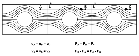
For viscous flows, the pressure is not periodic in the sense of Equation 1–20. Instead, the pressure drop between modules is periodic:
 | (1–21) |
If one of the density-based solvers is used,  is specified as a constant value. For the pressure-based solver, the local
pressure gradient can be decomposed into two parts: the gradient of a periodic component,
is specified as a constant value. For the pressure-based solver, the local
pressure gradient can be decomposed into two parts: the gradient of a periodic component,
 , and the gradient of a linearly-varying component,
  :
:
 | (1–22) |
where  is the periodic pressure and
  is the linearly-varying component of the pressure. The periodic pressure is
the pressure left over after subtracting out the linearly-varying pressure. The
linearly-varying component of the pressure results in a force acting on the fluid in the
momentum equations. Because the value of
is the linearly-varying component of the pressure. The periodic pressure is
the pressure left over after subtracting out the linearly-varying pressure. The
linearly-varying component of the pressure results in a force acting on the fluid in the
momentum equations. Because the value of  is not known a priori, it must be iterated on until the mass flow rate that
you have defined is achieved in the computational model. This correction of
is not known a priori, it must be iterated on until the mass flow rate that
you have defined is achieved in the computational model. This correction of  occurs in the pressure correction step of the SIMPLE, SIMPLEC, or PISO
algorithm where the value of
occurs in the pressure correction step of the SIMPLE, SIMPLEC, or PISO
algorithm where the value of  is updated based on the difference between the desired mass flow rate and the
actual one. You have some control over the number of sub-iterations used to update
is updated based on the difference between the desired mass flow rate and the
actual one. You have some control over the number of sub-iterations used to update
 . For more information about setting up parameters for
  in Ansys Fluent, see Setting Parameters for the Calculation of β in the Fluent User's Guide.
Note: Because streamwise-periodic flows are "fully developed", the resulting pressure gradient at convergence will only consist of it's linear component. Therefore, the calculated pressure field will not represent a physical pressure.
Integration of Equation 1–21, gives the static pressure for translational periodic flow as:
 | (1–23) |