


Predicting drop/wall impingement is not straightforward because of the large number of parameters involved. The outcome of any impingement is governed by the properties of the droplet liquid (viscosity, surface tension, and density) and by the impingement conditions (droplet diameter and droplet velocity). The two other important factors that contribute to the impingement outcome are the surface roughness and the thickness of the liquid film on the surface. In addition, wall temperature may also have an effect on impinging dynamics.
There are several models that represent impingement physics and predict the impingement outcome. Ansys Fluent provides the following models:
The Stanton and Rutland model [629], [631] uses the wall temperature and a Weber number-based criterion to define fixed value thresholds between the impingement regimes (stick, rebound, spread, and splash). In Fluent implementation, the original Stanton-Rutland model has been extended using the concepts from O’Rourke and Amsden [495]. See The Stanton-Rutland Model for more details.
The Kuhnke model [324] considers both dry and wet walls and takes into account, in addition to the drop properties and impingement conditions, the influence of surface roughness and film thickness. The Kuhnke model distinguishes between the following regimes: rebound, spread, splash, and dry splash (thermal breakup). For more information, see The Kuhnke Model.
The Stochastic Kuhnke model [606], [37] is derived from the Kuhnke model and has the following features:
Uses different regime transition criteria that have been developed and tuned for Selective Catalytic Reduction (SCR) modeling applications.
Includes stochastic effects into the critical temperature transition process.
Introduces the evaporative splash regime with the “partial evaporation” concept, where a fraction of the impinging droplets is assumed to completely vaporize under certain conditions.
See The Stochastic Kuhnke Model for details.
The user-defined Impingement Model can be employed through the use of
DEFINE_IMPINGEMENT,DEFINE_FILM_REGIMEandDEFINE_SPLASHING_DISTRIBUTIONuser-defined functions as described in User-Defined Functions in the Fluent User's Guide and in the Fluent Customization Manual.
Note:
The Lagrangian wall film model is available for the cases where energy equation is not solved with the below assumptions for the impingement/splashing models:
The wall temperature is 300 K
The saturation temperature of the liquid film is equal to 5000 K
The particle velocities referred in the sections that follow are relative to the frame of the wall. Dimensionless parameters
 and
and  are based on particle velocities normal to the wall unless specified.
The wall interaction is based on the work of Stanton [629] and O’Rourke [496], where the regimes are calculated for a drop-wall interaction based on local information. The four regimes (stick, rebound, spread, and splash) are based on the impact energy and wall temperature. The following chart is helpful in showing the cutoffs.
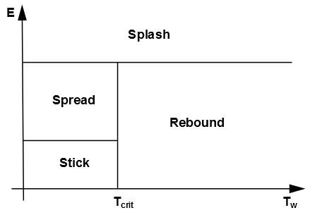
Below the critical transition temperature of the liquid, the impinging droplet can either stick, spread or splash, while above the critical transition temperature, the particle can either rebound or splash.
The criteria by which the regimes are partitioned are based on the impact energy and the critical transition temperature of the liquid. The impact energy is defined by
 | (12–208) |
where  is particle velocity normal to the wall,
  is the liquid density,
  is the diameter of the droplet,
  is the surface tension of the liquid, and
  is the film height. Here,
  is a boundary layer thickness, defined by
 | (12–209) |
where the Reynolds number is defined as  . By defining the energy as in Equation 12–208, the presence of the film on the wall suppresses the splash, but does not give unphysical results when the film height approaches zero.
The critical transition temperature is defined as:
 | (12–210) |
where  is the saturation temperature, and
  is the critical temperature factor with values between
1 and 1.5 depending on the application. The default value for
is the critical temperature factor with values between
1 and 1.5 depending on the application. The default value for  is 1; as a result, the default critical transition
temperature
is 1; as a result, the default critical transition
temperature  will be equal to the saturation temperature
of the droplet liquid
will be equal to the saturation temperature
of the droplet liquid  .
.
As an alternative for the Lagrangian wall film model, the critical transition temperature
 can be calculated from the saturation temperature of the liquid
 by adding a constant offset
  :
:
 | (12–211) |
The sticking regime is applied when the dimensionless energy  is less than 16, and the
particle velocity is set equal to the wall velocity. In the spreading
regime, the initial direction and velocity of the particle are set
using the wall-jet model, where the probability of the drop having
a particular direction along the surface is given by an analogy of
an inviscid liquid jet with an empirically defined radial dependence
for the momentum flux.
is less than 16, and the
particle velocity is set equal to the wall velocity. In the spreading
regime, the initial direction and velocity of the particle are set
using the wall-jet model, where the probability of the drop having
a particular direction along the surface is given by an analogy of
an inviscid liquid jet with an empirically defined radial dependence
for the momentum flux.
If the wall temperature is above the critical transition temperature of the liquid, impingement events below a critical impact energy ( ) results in the particles rebounding from the wall.
Splashing occurs when the impingement energy is above a critical
energy threshold, defined as  . The number of
splashed droplet parcels is set in the Wall boundary
condition dialog box with a default number of 4, however, you can
select numbers between zero and ten. The splashing algorithm follows
that described by Stanton [629] and is detailed
in Splashing.
. The number of
splashed droplet parcels is set in the Wall boundary
condition dialog box with a default number of 4, however, you can
select numbers between zero and ten. The splashing algorithm follows
that described by Stanton [629] and is detailed
in Splashing.
In the rebound regime, the velocity of the rebounding particle is given by:
 | (12–212) |
 | (12–213) |
where  and
and  are the tangential and normal components of the rebounding velocity,
  is the tangential component of the impinging velocity, and
  is the normal restitution coefficient given by:
 | (12–214) |
where  is the impingement angle in radians as measured from the wall surface.
The deviation angle of the rebounding particle,  , takes a random value between -90° and 90° from the incident direction.
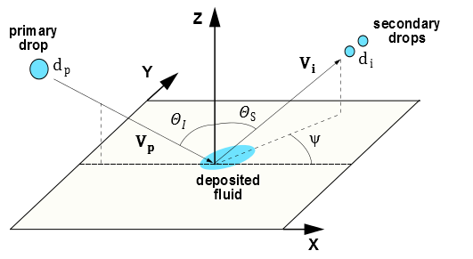
Figure 12.9: The Stanton-Rutland Model: Impinging and Splashing graphically depicts the following splashed droplet variables for the Stanton-Rutland splashing model.
Diameter of the impinging particle,

Impinging particle velocity,
 plus variability
Diameters of the splashed secondary particles,

Velocities of the splashed secondary particle

Impingement angle
 measured from the wall surface normal
Reflection angle of the splashed particle
 measured from the wall surface normal
Deviation angle
 from the incident direction
If the particle impinging on the surface has a sufficiently high energy, the particle splashes and several new particles are created. You can explicitly set the number of particles created by each impact in the DPM tab or the Wall Film tab of the Wall boundary condition dialog box. The minimum number of splashed parcels is three. The properties (diameter, magnitude, and direction) of the splashed parcels are randomly sampled from the experimentally obtained distribution functions described in the following sections. Setting the number of splashed parcels to zero in the Lagrangian wall film model turns off the splashing calculation for the Lagrangian model. Bear in mind that each splashed parcel can be considered a discrete sample of the distribution curves and that selecting the number of splashed drops in the Wall boundary condition dialog box does not limit the number of splashed drops, only the number of parcels representing those drops.
Therefore, for each splashed parcel, a different diameter is obtained by sampling a cumulative probability distribution function (CPDF), also referred to as F, which is obtained from a Weibull distribution function and fitted to the data from Mundo, et al. [465]. The equation is
 | (12–215) |
and it represents the probability of finding drops of diameter  in a sample of splashed drops. This distribution is similar to the Nakamura-Tanasawa distribution function used by O’Rourke [496] with distribution parameter
  . To ensure that the distribution functions produce physical results with an increasing Weber number, the following expression for
  from O’Rourke [496] is used. The ratio of the particle diameter at the peak of the splashed size distribution to the impinging particle diameter is given by
 | (12–216) |
where the expression for energy is given by Equation 12–208. Low Weber number impacts are described by the second term in Equation 12–216 and the peak splashed diameter ratio is never less than 0.06 for very high energy impacts in any of the experiments analyzed by O’Rourke [496]. The Weber number in Equation 12–216 is defined using normal particle velocity and diameter:
 | (12–217) |
The cumulative probability distribution function (CPDF) is needed so that a diameter can be sampled from the experimental data. The CPDF is obtained from integrating Equation 12–215 to obtain
 | (12–218) |
which is bounded by zero and one. An expression for the diameter (which is a function of  , the impingement Weber number
  , and the impingement energy) is obtained by inverting Equation 12–218 and sampling the CPDF between zero and one. The expression for the diameter of the
  splashed parcel is therefore given by
  where
where  is the
  random sample. Once the diameter of the splashed drop has been determined, the probability of finding that drop in a given sample is determined by evaluating Equation 12–215 at the given diameter.
In order to prevent the splashed particle diameter from becoming too large, Ansys Fluent uses distribution-limiting methods:
The tail limiting method (default for the Lagrangian Wall Film model) restricts the ratio
where
 is the particle diameter at 99.9% of CPDF.
The peak limiting method (default for the Eulerian Wall Film model) restricts the ratio
where
 is a limiting value ranging from 0.2 to 0.3 (default 0.22) as determined from the experimental data by Mundo [465].


The limiting method and parameter  can be selected through the text user interface (TUI) commands.
The number of droplets in each parcel is proportional to the value of the PDF for that droplet size. The total number of particles is then determined by the total mass that is splashed.
The mass fraction of the splashed particle  is obtained from the experimental data by Yarin and Weiss [724]. The splashed mass fraction expression by O’Rourke et al. [496] is given by:
 | (12–219) |
The splash mass fraction expression from Stanton et al. [629] is given by:
 | (12–220) |
where  is the non-dimensional impact velocity defined as:
 | (12–221) |
with  defined by Equation 12–236 and the constant
  taking the value of 2.37.
The splash mass fraction method can be selected through the TUI command, with the O’Rourke expression as default for Lagrangian Wall Film (LWF) and the Stanton expression as default for the Eulerian Wall Film (EWF).
The authors (O’Rourke et al. [496]) noted that nearly all of the impacts for typical diesel sprays are well above the upper bound and so the splashing event nearly always ejects 75% of the mass of the impinging drop. To obtain an expression for the total number of drops, we note that overall conservation of mass requires that the sum of the total mass of the splashed parcel(s) must equal the splashed mass fraction, or
 | (12–222) |
where  is the total mass of the impinging parcel. The expression for the total
number of splashed drops is
is the total mass of the impinging parcel. The expression for the total
number of splashed drops is
 | (12–223) |
The number of splashed drops per parcel is then determined by  multiplied
by the value of the PDF for that droplet size.
multiplied
by the value of the PDF for that droplet size.
To calculate the velocity with which the splashed drops leave the surface, additional correlations are sampled for the normal component of the velocity. A Weibull function, fit to the data from Mundo [465], is used as the PDF for the normal component. The probability density is given by
 | (12–224) |
where the index  refers to the
  th splashed droplet, and the subscript
  refers to the impinging droplet. The terms
  and
and  are functions of
  , the impingement angle measured from the surface normal:


The tangential component of the velocity is obtained from the
expression for the reflection angle  :
:
 | (12–225) |
combined with
 | (12–226) |
Note that the reflection angle  is measured from the surface normal, and both
  and
and  are in degrees.
The azimuthal angle  for the splashed droplets is computed according
to [630] assuming that it follows the distribution
for the splashed droplets is computed according
to [630] assuming that it follows the distribution  (Equation 12–227). The treatment is based on the approach
developed by Naber and Reitz [468].
(Equation 12–227). The treatment is based on the approach
developed by Naber and Reitz [468].
 | (12–227) |
where  is a parameter related to the impingement angle
  by:
by:
 | (12–228) |
 is determined by integrating Equation 12–227 and Equation 12–228 as follows:


In the above equations,  is a uniformly distributed random number between
0 and 1:
is a uniformly distributed random number between
0 and 1:

Finally, an energy balance is performed for the new parcels so that the sum of the kinetic and surface energies of the new drops does not exceed that of the old drops. The energy balance is given by
 | (12–231) |
where  is the threshold energy for splashing to occur. To ensure conservation
of energy, the following correction factor is computed:
is the threshold energy for splashing to occur. To ensure conservation
of energy, the following correction factor is computed:
 | (12–232) |
The threshold energy  is computed as:
 | (12–233) |
where  is the splashing threshold velocity computed from the critical Weber number as
 | (12–234) |
and the critical Weber number is given by:
 | (12–235) |
This correction factor is needed due to the relatively small number of sampled points for the velocity of the splashed drops (see Stanton [631] for more detail). The components of the splashed parcel are multiplied by the square root of  in Equation 12–232 so that energy will be conserved. The normal and tangential velocity components of the splashed parcels are therefore given by

It is important to note that splashing events are inherently transient, so the splashing submodel is only available with unsteady tracking in Ansys Fluent. Splashing can also cause large increases in source terms in the cells in which it occurs, which can cause difficulty in convergence between time steps. Thus, it may be necessary to use a smaller time step during the simulation when splashing is enabled.
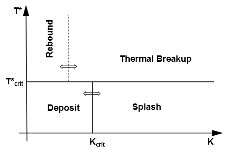
Figure 12.10: The Kuhnke Impingement Model Regimes shows the impingement
map for the Kuhnke [324] impingement model. The
model considers all relevant impingement phenomena by classifying
them into four regimes based on the dimensionless variables  and
and  : spread (or deposition),
rebound, splash, and dry splash (thermal breakup). The deposition
and splash regimes lead to formation of a wall film.
: spread (or deposition),
rebound, splash, and dry splash (thermal breakup). The deposition
and splash regimes lead to formation of a wall film.
The dimensionless variable  is defined as:
 | (12–236) |
where:
 | (12–237) |
 | (12–238) |
The dimensionless variable  is defined as:
 | (12–239) |
In the above equations, the following notation is used:
 = Weber number based on normal impingement velocity = Weber number based on normal impingement velocity | |
 = Laplace number = Laplace number | |
 = droplet density (kg/m3) = droplet density (kg/m3) | |
 = droplet diameter = droplet diameter | |
 = normal impingement velocity (m/s) = normal impingement velocity (m/s) | |
 = droplet surface tension
(N/m) = droplet surface tension
(N/m) | |
 = droplet viscosity (kg/m-s) = droplet viscosity (kg/m-s) | |
 = wall temperature (K) = wall temperature (K) | |
 = droplet saturation
temperature (K) = droplet saturation
temperature (K) |
When the wall temperature reaches the critical transition temperature , which marks the onset of film deposition, Equation 12–239
is used to define the critical temperature factor  :
:
 | (12–240) |
More specifically, the Kuhnke model considers the following regimes:
Spread: Adds the impinging drop to the wall film under one of the following conditions:
 and
and 
 and the wall is wet
Rebound: Emits the impinging drop without change in size under one of the following conditions:
 and
and 
 and the
wall is wet
and the
wall is wet
Splash: Atomizes drops into smaller ones if:

In the splashing regime, depending on the wall temperature and wall surface conditions, part of the impinging droplet mass may be deposited to form a film (splash), or the droplet may be completely atomized (dry splash or thermal breakup).
The critical transition parameters  and
and  are computed as follows.
The wall temperature-dependent transition is controlled by the
critical temperature factor  , which has values between 1.1 and 1.5 depending on the application.
The default value for
, which has values between 1.1 and 1.5 depending on the application.
The default value for  is 1;
as a result, the default critical transition temperature
is 1;
as a result, the default critical transition temperature  will be
equal to the saturation temperature of the droplet liquid
will be
equal to the saturation temperature of the droplet liquid  . Kuhnke [324] recommends values of 1.1 for single drop impingement
and 1.16 for impingement of droplet chains. For most urea-water
slurries,
. Kuhnke [324] recommends values of 1.1 for single drop impingement
and 1.16 for impingement of droplet chains. For most urea-water
slurries,  is set
at 1.4 [66].
is set
at 1.4 [66].
As an alternative for the Lagrangian wall film model, the critical transition temperature
can be calculated from the saturation temperature of the liquid
by adding a constant offset :
 | (12–241) |
For SCR slurries, recommended values for  range between 167 and 207° C.
The two critical values of the parameter  (one corresponding to the transition
between rebound and thermal breakup at high temperatures,
(one corresponding to the transition
between rebound and thermal breakup at high temperatures,  , and the other corresponding
to the transition between deposition and splash at low temperatures,
, and the other corresponding
to the transition between deposition and splash at low temperatures,  ) depend
on several parameters and wall conditions (wet or dry) as further
described.
) depend
on several parameters and wall conditions (wet or dry) as further
described.
Wet wall

(12–242)
where the dimensionless film height
 is calculated as:
with
 as the film height [m] and
  as the droplet diameter [m].
The other parameters in Equation 12–242 are expressed as:

(12–243)

(12–244)

(12–245)
Here
 ,
,  ,
,  ,
,  ,
,  , and
, and  are constants with values shown in Equation 12–242.
Dry wall

(12–246)
where  = dimensionless surface roughness
 = surface roughness (m) (average of absolute distance
from mean)
= surface roughness (m) (average of absolute distance
from mean)and

(12–247)
with
where
 is the threshold transition value
of the blending function taken as 0.99 and
is the threshold transition value
of the blending function taken as 0.99 and  is the width of the blending zone.


The parameter  is randomly sampled between 20 and 40:
 | (12–248) |
where  is a uniformly distributed random number between
0 and 1:
is a uniformly distributed random number between
0 and 1:

The parameter  is computed by the following
equations:
is computed by the following
equations:
 | (12–249) |
with

 | (12–250) |
| where | |
 = 54 = 54 | |
 = 130 = 130 | |
 = 13 = 13 |
The splashed mass fraction is determined as:
 | (12–251) |
where
 | (12–252) |
with 
In the rebound regime, the velocity of the rebounding particle is given by:
 | (12–253) |
 | (12–254) |
where  and
and  are the tangential and normal components of the rebounding velocity,
  is the tangential component of the impinging velocity, and
  is the normal restitution coefficient computed from:
 | (12–255) |
where  is the normal impact Weber number prior to impingement.
The deviation angle of the rebounding particle,  , takes a random value between -90° and 90° from the incident direction.
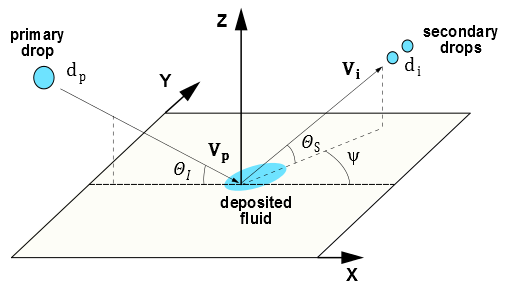
Figure 12.11: The Kuhnke Model: Impinging Drop graphically depicts the following splashed droplet variables for the Kuhnke splashing model:
Diameter of the impinging particle,
Impinging particle velocity,
 plus variability
Diameters of the splashed secondary particles,
Splashed particle mean velocity,
 plus variability
Impingement angle
measured from the wall surfaceReflection angle of the splashed particle
measured from the wall surfaceDeviation angle
from the incident direction
Note: Note that, conventionally, the impingement and reflection angles are measured differently within the Stanton/Rutland and Kuhnke model frameworks:
the Stanton and Rutland model: from the normal to the wall surface
the Kuhnke model: from the wall surface
The properties of the splashed particles are calculated as follows.
As a first step, the mean diameter of the splashed drops is computed from:
 | (12–256) |
with
 | (12–257) |
where
 = diameter of primary drop [m] = diameter of primary drop [m] | |
 = normal impact Weber number of the impingement particle = normal impact Weber number of the impingement particle | |
 = impingement angle in radians = impingement angle in radians |
Next, as originally proposed by Stanton and Rutland [629], [631], the splashed drop diameters  are randomly sampled from the inverse of a continuous Weibull Probability Density Function
  which is described by:
 | (12–258) |
with  =2. A limiting method as described in Splashing is also applied.
The number of droplets in each splashed parcel is determined from the overall mass balance by Equation 12–222.
The mean splashed droplet velocity  is calculated from the secondary Weber number
  and mean droplet size
  as:
as:
 | (12–259) |
where
 | (12–260) |
where  and
and  are based on absolute particle velocities, and
 = 0.85 = 0.85 | |

| |
 = 2 = 2 |
Similarly to the splashed droplet diameters, the splashed drop velocities  are randomly sampled from the inverse of a continuous Weibull Probability
Density Function with the distribution average value being
are randomly sampled from the inverse of a continuous Weibull Probability
Density Function with the distribution average value being  .
.
The ejection angle  is computed from the mean value
  by assuming a logistic distribution:
 | (12–261) |
where angles (in degrees) are distributed by the logistic PDF  with
with  =4.
=4.
The notation used here is as follows:
 = dimensionless surface roughness = dimensionless surface roughness 
| |
 = surface roughness (m) (average of maximal height differences) = surface roughness (m) (average of maximal height differences) |
The inverse of the continuous logistic PDF is given by:
 | (12–262) |
The deviation angle  is determined by:
 | (12–263) |
where

The regime map of the Stochastic Kuhnke model is shown in Figure 12.12: The Regime Map of the Stochastic Kuhnke Model.
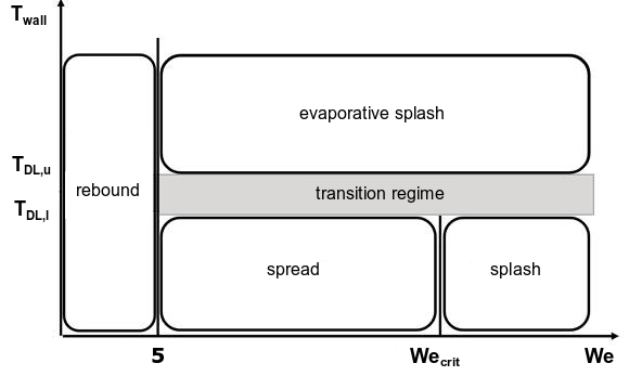
The model considers all relevant impingement phenomena by classifying them into the following four core regimes based on critical temperature and Weber number transition criteria:
rebound
spread
splash
evaporative splash
The spread and splash regimes lead to formation of a wall film. In addition, the transition regime is introduced to avoid abrupt changes during the film deposition process.
The regime transition criteria are defined as follows. A critical temperature range is
defined between the upper and lower deposition limits  and
and  :
:
 | (12–264) |
 | (12–265) |
where
 = liquid film saturation temperature [K] = liquid film saturation temperature [K] |
 = upper deposition limit offset [K] = upper deposition limit offset [K] |
 = deposition range temperature difference [K] = deposition range temperature difference [K] |
The Weber number criterion is defined differently for wet and dry walls:


In Equation 12–266 and Equation 12–267:
 = Laplace number = Laplace number |
 = Laplace number constant = Laplace number constant |
 = function of wall roughness = function of wall roughness  interpolated from Table 12.2: Parameter A as a Function of Wall Roughness interpolated from Table 12.2: Parameter A as a Function of Wall Roughness
|
Table 12.2: Parameter A as a Function of Wall Roughness
 (microns) (microns) |

|
| 0.05 | 5264 |
| 0.14 | 4534 |
| 0.84 | 2634 |
| 3.1 | 2056 |
| 12 | 1322 |
The Laplace number is expressed as:
 | (12–268) |
where
 = droplet density = droplet density |
 = droplet surface tension = droplet surface tension |
 = droplet diameter = droplet diameter |
 = droplet viscosity = droplet viscosity |
Finally, the Stochastic Kuhnke model assigns the appropriate regime for each impingement event according to the droplet Weber number (see the definition of the Weber number in section "The Kuhnke Model" in the Ansys Fluent Theory Guide) and the wall conditions. These regimes are:
Rebound
Regime boundaries:
 and
and 
The impinging drop is emitted without change in size. The velocity components of the rebounding particle are calculated in accordance with section "Rebound" for the Kuhnke model in the Ansys Fluent Theory Guide.
Spread
Regime boundaries:
 and
and 
The impinging drop is added to the wall film.
Splash
Regime boundaries:
 and
and 
Part of the impinging droplet mass is deposited to form a film, and the rest of the droplet is atomized. The splashed mass fraction and the splashed droplet variables are computed according to section "Splashing" for the Kuhnke model in the Ansys Fluent Theory Guide.
Evaporative Splash
Regime boundaries:
 and
and 
A small fraction of the impinging liquid spray is assumed to vaporize immediately upon impact, while the rest is completely atomized emitting smaller sized droplets. The vaporization events occurring in this regime are controlled by random number sampling. Similarly to the splash regime, the splashed droplet variables are computed as described in section "Splashing" for the Kuhnke model in the Ansys Fluent Theory Guide.
Transition Regime
Regime boundaries:
 and
and 
Under these conditions, any of the regimes (spread, splash, or evaporative splash) may be assigned to the impinging drop. This is decided based on comparison of a random number with the deposition ratio
 computed from Equation 12–269 in combination with the
droplet Weber number and the wet or dry wall criterion.
computed from Equation 12–269 in combination with the
droplet Weber number and the wet or dry wall criterion.
(12–269)