Ansys Fluent is able to predict heat transfer in periodically repeating geometries, such as compact heat exchangers, by including only a single periodic module for analysis.
This section discusses streamwise-periodic heat transfer. The treatment of streamwise-periodic flows is discussed in Periodic Flows, and a description of no-pressure-drop periodic flow is provided in Periodic Boundary Conditions.
Information about streamwise-periodic heat transfer is presented in the following sections:
The following sections contain information about periodic heat transfer:
As discussed in Overview and Limitations,
streamwise-periodic flow conditions exist when the flow pattern repeats over
some length  , with a constant pressure drop across each repeating module
along the streamwise direction.
, with a constant pressure drop across each repeating module
along the streamwise direction.
Periodic thermal conditions may be established when the thermal boundary conditions are of the constant wall temperature or wall heat flux type. In such problems, the temperature field (when scaled in an appropriate manner) is periodically fully developed [116]. As for periodic flows, such problems can be analyzed by restricting the numerical model to a single module or periodic length.
In addition to the constraints for streamwise-periodic flow discussed in Limitations for Modeling Streamwise-Periodic Flow, the following constraints must be met when periodic heat transfer is to be considered:
The pressure-based solver must be used.
The thermal boundary conditions must be of the specified heat flux or constant wall temperature type. Furthermore, in a given problem, these thermal boundary types cannot be combined: all boundaries must be either constant temperature or specified heat flux. You can, however, include constant-temperature walls and zero-heat-flux walls in the same problem. For the constant-temperature case, all walls must be at the same temperature (profiles are not allowed) or zero heat flux. For the heat flux case, profiles and/or different values of heat flux may be specified at different walls.
When constant-temperature wall boundaries are used, you cannot include viscous heating effects or any volumetric heat sources.
In cases that involve solid regions, the regions cannot straddle the periodic plane.
The thermodynamic and transport properties of the fluid (heat capacity, thermal conductivity, viscosity, and density) cannot be functions of temperature. (You cannot, therefore, model reacting flows.) Transport properties may, however, vary spatially in a periodic manner, and this allows you to model periodic turbulent flows in which the effective turbulent transport properties (effective conductivity, effective viscosity) vary with the (periodic) turbulence field.
The periodic boundary condition with specified non-zero mass flow rate and/or pressure gradient cannot be used for variable density flows.
Theory and Using Periodic Heat Transfer provide more detailed descriptions of the input requirements for periodic heat transfer.
Streamwise-periodic flow with heat transfer from constant-temperature walls is one of two classes of periodic heat transfer that can be modeled by Ansys Fluent. A periodic fully developed temperature field can also be obtained when heat flux conditions are specified. In such cases, the temperature change between periodic boundaries becomes constant and can be related to the net heat addition from the boundaries as described in this section.
Important: Periodic heat transfer can be modeled only if you are using the pressure-based solver.
For the case of constant wall temperature, as the fluid flows through the periodic domain, its temperature approaches that of the wall boundaries. However, the temperature can be scaled in such a way that it behaves in a periodic manner. A suitable scaling of the temperature for periodic flows with constant-temperature walls is [116]
 | (16–17) |
The bulk temperature,  , is defined by
 | (16–18) |
where the integral is taken over the inlet periodic boundary ( ). It is the scaled temperature,
  , which obeys a periodic condition across the domain of length
 .
.
When periodic heat transfer with heat flux conditions is considered, the form of the unscaled temperature field becomes analogous to that of the pressure field in a periodic flow:
 | (16–19) |
where  is the periodic length vector of the domain. This temperature
gradient,
is the periodic length vector of the domain. This temperature
gradient,  , can be written in terms of the total heat addition within the
domain,
, can be written in terms of the total heat addition within the
domain,  , as
, as
 | (16–20) |
where  is the specified or calculated mass flow rate.
A typical calculation involving both streamwise-periodic flow and periodic heat transfer is performed in two parts. First, the periodic velocity field is calculated (to convergence) without consideration of the temperature field. Next, the velocity field is frozen and the resulting temperature field is calculated. These periodic flow calculations are accomplished using the following procedure:
Set up a mesh with translationally periodic boundary conditions.
Specify constant thermodynamic and molecular transport properties.
Specify either the periodic pressure gradient or the net mass flow rate through the periodic boundaries.
Compute the periodic flow field, solving momentum, continuity, and (optionally) turbulence equations.
Specify the thermal boundary conditions at walls as either heat flux or constant temperature.
Define an inlet bulk temperature.
Solve the energy equation (only) to predict the periodic temperature field.
In order to model the periodic heat transfer, you will need to set up your periodic model in the manner described in User Inputs for the Pressure-Based Solver for periodic flow models with the pressure-based solver, noting the restrictions discussed in Limitations for Modeling Streamwise-Periodic Flow and Constraints for Periodic Heat Transfer Predictions. In addition, you will need to provide the following inputs related to the heat transfer model:
Enable the solution of the energy equation by right-clicking Energy in the tree (under Setup/Models) and clicking On in the menu that opens (Figure 16.1: Enabling the Energy Equation).
 Setup →
Models → Energy
Setup →
Models → Energy
 On
On
Define the thermal boundary conditions according to one of the following procedures. The boundary condition dialog boxes can be opened by right-clicking the boundary name in the tree (under Setup/Boundary Conditions) and clicking Edit... in the menu that opens; alternatively, you can open them from the Boundary Conditions task page:
Setup →  Boundary Conditions
If you are modeling periodic heat transfer with specified-temperature boundary conditions, set the wall temperature
 for all wall boundaries in their respective
Wall dialog box. Note that all wall
boundaries must be assigned the same temperature and that the entire
domain (except the periodic boundaries) must be
“enclosed” by this fixed-temperature condition, or by
symmetry or adiabatic (
for all wall boundaries in their respective
Wall dialog box. Note that all wall
boundaries must be assigned the same temperature and that the entire
domain (except the periodic boundaries) must be
“enclosed” by this fixed-temperature condition, or by
symmetry or adiabatic ( =0) boundaries.
If you are modeling periodic heat transfer with specified-heat-flux boundary conditions, set the wall heat flux in the Wall dialog box for each wall boundary. You can define different values of heat flux on different wall boundaries, but you should have no other types of thermal boundary conditions active in the domain.
Define solid regions, if appropriate, according to one of the following procedures. The cell zones can be defined by right-clicking the zone name in the tree (under Setup/Cell Zone Conditions), or using the Cell Zone Conditions task page:
Setup → Cell
Zone Conditions
If you are modeling periodic heat transfer with specified-temperature conditions, conducting solid regions can be used within the domain, provided that on the perimeter of the domain they are enclosed by the fixed-temperature condition. Heat generation within the solid regions is not allowed when you are solving periodic heat transfer with fixed-temperature conditions.
If you are modeling periodic heat transfer with specified-heat-flux conditions, you can define conducting solid regions at any location within the domain, including volumetric heat addition within the solid, if desired.
Set constant material properties (density, heat capacity, viscosity, thermal conductivity), not temperature-dependent properties, using the Create/Edit Materials dialog box. This dialog box can be opened by right-clicking the material name in the tree (under Setup/Materials) and clicking Edit... in the menu that opens; alternatively, you can open them from the Materials task page:
Setup →
Materials
Specify the Upstream Bulk Temperature in the Periodic Conditions dialog box, which can be opened from Boundary Conditions task page:
Setup →
Boundary Conditions → Periodic
Conditions...
Important: If you are modeling periodic heat transfer with specified-temperature conditions, the bulk temperature should not be equal to the wall temperature, since this will give you the trivial solution of constant temperature everywhere.
Set the solution parameters as described in Solution Strategies for Periodic Heat Transfer.
Run the solution and monitor the convergence as described in Monitoring Convergence.
Postprocess the results as described in Postprocessing for Periodic Heat Transfer.
After completing the inputs described in Using Periodic Heat Transfer, you can solve the flow and heat transfer problem to convergence. The most efficient approach to the solution, however, is a sequential one in which the periodic flow is first solved without heat transfer and then the heat transfer is solved leaving the flow field unaltered. This sequential approach is accomplished as follows:
Disable solution of the energy equation in the Equations dialog box; this dialog box is accessed by right-clicking Solution Controls in the tree (under Solution) and clicking Equations... in the menu that opens.
Solution →
Controls
Equations...
Solve the remaining equations (continuity, momentum, and, optionally, turbulence parameters) to convergence to obtain the periodic flow field.
Important: When you initialize the flow field before beginning the calculation, use the mean value between the inlet bulk temperature and the wall temperature for the initialization of the temperature field.
Return to the Equations dialog box and turn off solution of the flow equations and turn on the energy solution.
Solve the energy equation to convergence to obtain the periodic temperature field of interest.
While you can solve your periodic flow and heat transfer problems by considering both the flow and heat transfer simultaneously, you will find that the procedure outlined above is more efficient.
If you are modeling periodic heat transfer with specified-temperature conditions, you can monitor the value of the bulk temperature ratio
 | (16–21) |
during the calculation by creating a report plot that includes bulk temperature ratio (periodic-bulk-temperature-ratio), to ensure that you reach a converged solution. See Monitoring Statistics for additional information.
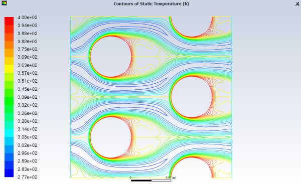
The actual temperature field predicted by Ansys Fluent in periodic models will not be
periodic, and viewing the temperature results during postprocessing will display
this actual temperature field ( of Equation 16–17). The displayed temperature
may exhibit values outside the range defined by the inlet bulk temperature and the
wall temperature. This is permissible since the actual temperature profile at the
inlet periodic face will have temperatures that are higher or lower than the inlet
bulk temperature.
of Equation 16–17). The displayed temperature
may exhibit values outside the range defined by the inlet bulk temperature and the
wall temperature. This is permissible since the actual temperature profile at the
inlet periodic face will have temperatures that are higher or lower than the inlet
bulk temperature.
Static Temperature is found in the Temperature... category of the variable selection drop-down list that appears in postprocessing dialog boxes.
Figure 16.59: Temperature Field in a 2D Heat Exchanger Geometry With Fixed Temperature Boundary Conditions shows the temperature field in a periodic heat exchanger geometry.
Figure 16.59: Temperature Field in a 2D Heat Exchanger Geometry With Fixed Temperature Boundary Conditions