


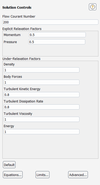
The Solution Controls task page allows you to set common solution parameters.
Important: This feature offers reduced functionality when running Fluent under the Pro capability level.
Controls
- Courant Number
sets the fine-grid Courant number (time step factor) when the density-based solver is used. See Changing the Courant Number for guidelines on setting the Courant number.
When the pressure-based solver is used for time-independent flows, and the Coupled pressure-velocity scheme is used, the Courant Number is used to stabilize the convergence behavior. See Under-Relaxation of Equations in the Theory Guide for a correlation of the under-relaxation factor and courant number.
- Flow Courant Number
sets the Courant number for multiphase flow using the pressure-based coupled solver. The Flow Courant Number is used to stabilize the convergence behavior.
- Volume Fraction Courant Number
sets the Courant number for multiphase flow using the pressure-based solver is coupled with the volume fraction. The default value is 200 and will appear in the interface when the Coupled with Volume Fraction option appears in the Solution Methods task page.
- Pseudo Time Courant Number
sets the pseudo time Courant number when a Pseudo Time Method is selected with a pressure-based segregated solver (see Local Time Step Method Setting).
- Explicit Relaxation Factors
for the Coupled scheme defines the explicit relaxation of variables between sub-iterations for momentum and pressure. See Under-Relaxation of Variables in the Theory Guide for information.
- Multigrid Levels
specifies the maximum number of coarse levels to be created by the FAS multigrid solver. This item is the same as the Max Coarse Levels under FAS Multigrid Controls in the Multigrid tab of the Advanced Solution Controls Dialog Box, and it appears only when the density-based explicit solver is used.
- Residual Smoothing
contains parameters that govern the use of implicit residual smoothing. (See Implicit Residual Smoothing in the Theory Guide and Using Residual Smoothing to Increase the Courant Number for details.) This section of the task page will appear only when the density-based explicit solver is used.
- Iterations
sets the number of iterations of the Jacobi smoother to use. If Iterations is 0, then no implicit residual smoothing is performed.
- Smoothing Factor
sets the implicit residual smoothing factor. This item will not appear unless Iterations is set to a non-zero value.
- Under-Relaxation Factors
contains the under-relaxation factors for all equations that are being solved with the pressure-based solver. (See Setting Under-Relaxation Factors for details.) In the field next to each equation, you can set the under-relaxation factor for that equation.
When one of the density-based solvers is used, Under-Relaxation Factors will appear only for the following variables, when they are included in your model: solid (for conjugate heat transfer models), turbulence variables, and viscosity. The solid under-relaxation factor is used to scale the CFL value in the solid region only if the under-relaxation value is set to a value less than 1. When the under-relaxation value is set to 1, then the solver ignores the specified CFL value for the solid and instead uses a very large value of CFL. This is done to speed up the convergence in the solid region. The density-based solvers use a segregated method to solve these equations; all the other equations are solved in a coupled manner, so there are no under-relaxation factors for them.
When Non-Iterative Time Advancement is selected for the pressure-based solver, the Non-Iterative Solver Relaxation Factors define the explicit relaxation (Under-Relaxation of Variables in the Theory Guide) of variables between sub-iterations and are used to prevent the solution from diverging.
Note the following if a Pseudo Time Method is selected: if Global Time Step is selected for steady-state cases with the pressure-based coupled solver or the density-based implicit solver, the Pseudo Time Explicit Relaxation Factors can be specified (see Global Time Step Method Settings); if Local Time Step is selected for a pressure-based segregated solver, the Pseudo Time Under-Relaxation Factors can be specified (see Local Time Step Method Setting).
- Acoustics Wave Equation Solver Controls
contains parameters that govern the acoustics wave equation solver
- Relative Convergence Criterion
sets the relative convergence criterion for the acoustics wave equation solver.
- Max Iteration/Time Step
sets the maximum number of iterations per time step.
- Default
sets the fields to their default values, as assigned by Ansys Fluent.
- Equations...
displays the Equations Dialog Box.
- Limits...
displays the Solution Limits Dialog Box.
- Advanced...
displays the Advanced Solution Controls Dialog Box.
- Set All Species URFs Together
enables an option to use the same under-relaxation factors for all the species rather than setting each of the species individually. Notice that you will no longer see your list of individual species, instead a Species field will appear with the specified under-relaxation factor. Note that this option is available when species transport is enabled.
For additional information, see the following sections:
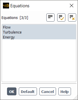
The Equations dialog box contains a list of the equations being solved for the current model. To temporarily disable solution of an equation, deselect it in this list and click . To re-enable the calculation for an equation, select it and click . See Step-by-Step Solution Processes for details about using this feature in a step-by-step solution process.
Note that, when one of the density-based solvers is used, Energy will not appear as a separate item in the Equations list. For the density-based solvers the energy equation is included in the Flow category (which also includes the pressure and momentum equations).
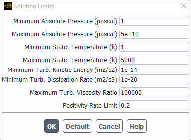
The Solution Limits dialog box allows you to improve the stability of the solution. See Setting Solution Limits for details about the items below.
Controls
- Minimum Absolute Pressure, Maximum Absolute Pressure
set the limiting minimum and maximum allowable values for absolute pressure.
- Minimum Static Temperature, Maximum Static Temperature
set the limiting minimum and maximum allowable values for temperature.
- Minimum Turb. Kinetic Energy
sets the limiting minimum value of turbulent kinetic energy (
 ) in the flow field. This parameter appears when
one of the
) in the flow field. This parameter appears when
one of the  -
-  or
or  -
-  models or the RSM is
used.
models or the RSM is
used.- Minimum Turb. Dissipation Rate
sets the limiting minimum value of turbulent dissipation rate (
 ) in the flow field. This parameter appears
when one of the
) in the flow field. This parameter appears
when one of the  -
-  models or the RSM is used.
- Minimum Spec. Dissipation Rate
sets the limiting minimum value of specific dissipation rate (
 ) in the flow field. This parameter appears
when one of the
) in the flow field. This parameter appears
when one of the  -
-  models is used.
- Maximum Turb. Viscosity Ratio
sets the limiting maximum allowable value of the ratio of turbulent to laminar viscosity (
 ). The turbulent viscosity is reduced to the necessary
value so as not to exceed the maximum allowable viscosity ratio.
). The turbulent viscosity is reduced to the necessary
value so as not to exceed the maximum allowable viscosity ratio.This parameter appears for all turbulent flows.
- Minimum Vol. Frac. for Matrix Solution
sets the limiting minimum value for volume fraction in the matrix solution. This field appears for Eulerian multiphase simulations run on a double-precision solver.
- Positivity Rate Limit
sets the limiting value for the rate of reduction of temperature. See Adjusting the Positivity Rate Limit for details.
This item appears only when one of the density-based solvers is used.
- Default
sets the fields to their default values, as assigned by Ansys Fluent. After execution, the Default button becomes the Reset button.
- Reset
resets the fields to their most recently saved values (for example, the values before Default was selected). After execution, the Reset button becomes the Default button.
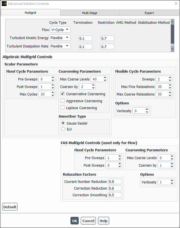
The Advanced Solution Controls dialog box allows you to set parameters related to the multigrid, multi-stage, and non-iterative solvers.
Controls
- Multigrid
tab contains parameters related to the multigrid solver. See Modifying Algebraic Multigrid Parameters and Setting FAS Multigrid Parameters for details about the items below.
- Cycle Type
contains a drop-down list for each equation that is being solved. From this list you can select the multigrid cycle type (Flexible, V-Cycle, W-Cycle, or F-Cycle). See Specifying the Multigrid Cycle Type for details.
Note that, for the density-based solvers, the Pressure, Momentum, and Energy equations will not appear individually. They will instead be grouped together and called Flow.
Furthermore, for the density-based explicit solver, the Cycle Type choices for the Flow equations will be limited to V-Cycle and W-Cycle, while the choices for Flow for the density-based implicit solver will be limited to V-Cycle and F-Cycle.
- Termination
specifies the termination criterion for each equation that is being solved using algebraic multigrid. See Setting the Termination and Residual Reduction Parameters for details.
- Restriction
specifies the residual reduction criterion for each equation that is being solved using the Flexible algebraic multigrid cycle. See Setting the Termination and Residual Reduction Parameters for details. (This item will not appear for an equation that is using a V-Cycle, W-Cycle, or F-Cycle.)
- Stabilization Method
contains the drop-down list to choose the stabilization method. For further details, see Setting the Stabilization Method.
- BCGSTAB
enables the bi-conjugate gradient stabilized method.
- RPM
enables the recursive projection method. RPM stabilization is mainly used in conjunction with the coupled pressure-based solver.
- CG
enables the conjugate gradient method. CG stabilization is mainly used in conjunction with the segregated pressure-based solver.
- GMRES
enables the generalized minimal residual method. GMRES stabilization is recommended for cases that fail to converge with the BCGSTAB method.
- Algebraic Multigrid Controls
contains parameters related to the algebraic multigrid solver. See Algebraic Multigrid (AMG) in the Theory Guide and Modifying Algebraic Multigrid Parameters for details.
- Scalar and Coupled Parameters
contain parameters that you can set, If you are using the density-based explicit solver or the pressure-based solver with any of the segregated schemes, described in Pressure-Velocity Coupling in the Theory Guide and Choosing the Pressure-Velocity Coupling Method, you will only set Scalar Parameters. If you are using the density-based implicit or the pressure-based coupled scheme, described in Coupled Algorithm, then you can set the Coupled Parameters.
- Fixed Cycle Parameters
contains parameters that control the V, W, and F cycles. You can set the number of Pre-Sweeps and Post-Sweeps, and the Max Cycles. Normally one post-sweep is performed and no pre-sweeps are done. See Fixed Cycle Parameters for details about using the items below.
- Pre-Sweeps
sets the number of sweeps to perform before moving to a coarser level.
- Post-Sweeps
sets the number of sweeps to perform after coarser level corrections have been applied.
- Max Cycles
sets the maximum number of V, W, or F cycles to be performed. The multigrid solver will continue to solve the set of equations until either the maximum number of cycles has been performed, or the Termination criteria are satisfied.
- Coarsening Parameters
contains parameters that control the grouping of equations in the algebraic multigrid algorithm. See Coarsening Parameters for details
- Max Coarse Levels
is the maximum number of coarse levels that will be built by the multigrid solver. Sets of coarser simultaneous equations are built until the maximum number of levels has been created, or the coarsest level has only 3 equations. Each level has about half as many unknowns as the previous level, so coarsening until there are only a few nodes left will require about as much total coarse-level coefficient storage as was required on the fine mesh. Reducing the maximum coarse levels will reduce the memory requirements, but may require more iterations to achieve a converged solution. Setting Max Coarse Levels to 0 turns off the multigrid solver.
- Coarsen by
controls the number of equations on each successively coarser grid level. By default, this parameter is set to 2, indicating that the number of equations on each level will be 1/2 of the number on the previous level. In general, the number of equations on each coarser grid level will be approximately equal to 1/
 of the number on the previous level, where
  is the value set for the Coarsen by
parameter.
is the value set for the Coarsen by
parameter.- Conservative Coarsening
enables the use of conservative coarsening techniques that can improve parallel performance and/or convergence for some difficult cases.
- Aggressive Coarsening
specifies the use of a version of the AMG solver that is optimized for high coarsening rates. It is recommended if the AMG solver diverges with the default settings.
- Laplace Coarsening
enables the use of Laplace coefficients when grouping cells for coarsening.
- Smoother Type
consist of two types:
- Gauss-Seidel
is the simplest smoother type and is recommended when using the pressure-based segregated solver.
- ILU
is more CPU intensive, but has better smoothing properties for block-coupled systems such as the pressure-based coupled solver and the density-based implicit solver.
- Flexible Cycle Parameters
contains parameters that control the flexible multigrid cycle.
- Sweeps
specifies the number of times to apply the smoothing method each time a relaxation is performed.
- Max Fine Relaxations
sets the maximum number of relaxations to be performed on the Level 1 grid (fine grid level). This parameter eliminates the possibility that the Gauss-Seidel solver will get "stuck" on the fine grid level, unable to reduce the residuals by the fraction (
 ) required by the Termination criteria.
- Max Coarse Relaxations
sets the maximum number of relaxations to be performed on each grid level above Level 1 (that is, the coarse grid levels). This parameter eliminates the possibility that the Gauss-Seidel solver will get "stuck" on a coarse grid level, unable to reduce the residuals on that level by the fraction (
 ) required by the Termination criteria. If the iterative solution on a given
grid level is unable to meet the accuracy constraint of the Termination criteria, the correction equation will be
deemed "converged" when this maximum number of relaxations
on that grid level has been performed.
) required by the Termination criteria. If the iterative solution on a given
grid level is unable to meet the accuracy constraint of the Termination criteria, the correction equation will be
deemed "converged" when this maximum number of relaxations
on that grid level has been performed.
- Options
contains additional multigrid parameters.
- Verbosity
controls the amount of information that is printed out by the multigrid solver for monitoring purposes. See Setting the Verbosity for details
- FAS Multigrid Controls
contains parameters related to the FAS multigrid solver. See Full-Approximation Storage (FAS) Multigrid in the Theory Guide and Setting FAS Multigrid Parameters for details. As noted in the title of this dialog box section, the FAS multigrid solver is used only for the Flow equations (pressure, momentum, and energy).
This section of the dialog box appears only when the density-based explicit solver is used.
- Fixed Cycle Parameters
contains parameters that control the V, W, and F cycles of the FAS multigrid solver.
- Pre-Sweeps
sets the number of iterations of the multi-stage solver to be performed on a given grid level before proceeding to a coarser grid level (the value of
 described
in Multigrid Cycles in the Theory Guide). Typically, this is set to 1.
described
in Multigrid Cycles in the Theory Guide). Typically, this is set to 1.- Post-Sweeps
sets the number of multigrid cycles to be performed on a given grid level before proceeding back up to the finer grid level (the value of
 described
in Multigrid Cycles in the Theory Guide). A value of 1 results in V-cycle multigrid, and a value of 2 results
in W-cycle multigrid.
described
in Multigrid Cycles in the Theory Guide). A value of 1 results in V-cycle multigrid, and a value of 2 results
in W-cycle multigrid.
- Coarsening Parameters
contains parameters that control the grouping of cells in the FAS multigrid algorithm.
- Max Coarse Levels
sets the maximum number of grid levels to be used in the multigrid process. A value of 0 disables multigrid (no coarse grid levels). If the coarse grids do not already exist, they are created automatically when you start iterating; you cannot create them by clicking the button. See Turning On FAS Multigrid for details.
- Coarsen by
controls the number of cells in each successively coarser grid level. By default, this parameter is set to 2, indicating that the number of cells on each level will be 1/2 of the number on the previous level. In general, the number of cells on each coarser grid level will be equal to 1/
 of the number on the previous level, where
  is the value set for the Coarsen by parameter.
- Relaxation Factors
are provided to moderate and stabilize the multigrid corrections.
- Courant Number Reduction
sets the factor by which to reduce the Courant number for coarse grid levels (that is, every level except the finest). Some reduction of time step (such as the default 0.9) is typically required because the stability limit cannot be determined as precisely on the irregularly shaped coarser grid cells.
- Correction Reduction
sets the factor by which to reduce the magnitude of the multigrid corrections transferred from one level to the next finer level. A typical value with
 is 0.6. If two Pre-Sweeps and two Post-Sweeps are
performed, this value can often be increased to 1.0 (that is, full
correction transfer).
is 0.6. If two Pre-Sweeps and two Post-Sweeps are
performed, this value can often be increased to 1.0 (that is, full
correction transfer).- Species Correction Reduction
sets the factor by which to reduce the magnitude of the species corrections to stabilize the multigrid calculation. This item appears only when species transport is being modeled.
- Correction Smoothing
sets the correction smoothing factor used to interpolate corrections from a coarser grid to a finer grid. For multigrid on structured meshes, corrections can be interpolated up to a finer mesh "smoothly" by using, for example, tri-linear interpolation. For unstructured meshes there is no analogous simple, algebraic procedure that can be used to interpolate without introducing substantial high frequency "noise". Instead, the corrections are first interpolated, and then subjected to a smoothing pass. The default Correction Smoothing value of 0.5 should be acceptable for all cases; you should not need to change it.
- Options
contains additional multigrid parameters.
- Verbosity
controls the amount of information that is printed out by the multigrid solver for monitoring purposes.
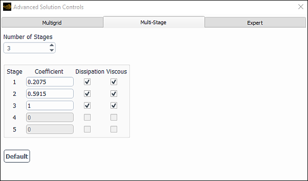
- Multi-Stage
tab allows you to set parameters that govern the operation of the multi-stage solver. It is available only when the density-based explicit solver is used. See Changing the Multi-Stage Scheme for details about the items below.
Controls
- Number of Stages
is the number of stages used in the multi-stage scheme. The default scheme is a 3-stage scheme with coefficients of 0.2075, 0.5915, and 1.0 for the first through third stages, respectively. Although the dialog box limits the maximum number of stages to five, you can define a scheme with an arbitrary number of stages with the
solve/set/multi-stagetext command.- Stage
labels the stage to which the parameters in the other columns apply.
- Coefficient
sets the multi-stage coefficient for each stage. Coefficients should be greater than zero and less than one. The final stage should always have a coefficient of 1.
- Dissipation
sets the stages for which artificial dissipation is evaluated. If a Dissipation box is selected for a particular stage, artificial dissipation will be updated on that stage. If not selected, artificial dissipation will remain "frozen" at the value of the previous stage.
- Viscous
sets the stages for which viscous stresses are evaluated. If a Viscous box is selected for a particular stage, viscous stresses will be updated on that stage. If not selected, viscous stresses will remain "frozen" at the value of the previous stage. Viscous stresses should always be computed on the first stage, and successive evaluations will increase the "robustness" of the solution process, but will also increase the expense (that is, increase the CPU time per iteration). For steady problems, the final solution is independent of the stages on which viscous stresses are updated.
- Default
sets the fields to their default values, as assigned by Ansys Fluent. After execution, the Default button becomes the Reset button.
- Reset
resets the fields to their most recently saved values (that is, the values before Default was selected). After execution, the Reset button becomes the Default button.
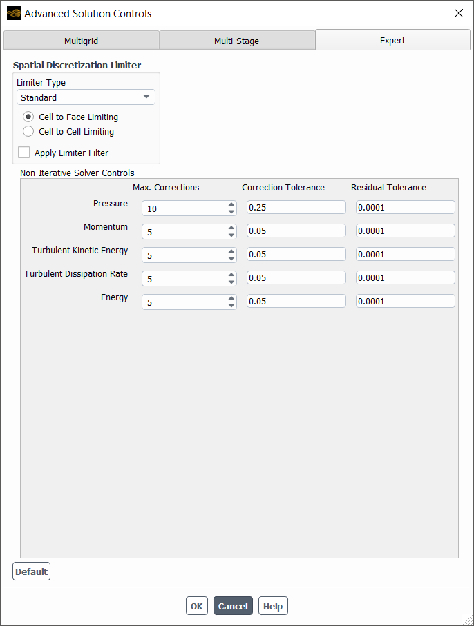
- Expert
tab contains specialized parameters for limiting spatial discretization, as well as controls for the non-iterative solver.
Controls
- Spatial Discretization Limiter
contains controls for limiting the spatial discretization. See Selecting Gradient Limiters for more information about limiters.
- Limiter Type
selects the type of limiter applied to the spatial discretization: Standard, Multidimensional, or Differentiable.
- Cell to Face Limiting
is where the limited value of the reconstruction gradient is determined at the cell face centers. This is the default method.
- Cell to Cell Limiting
is where the limited value of the reconstruction gradient is determined along a scaled line between two adjacent cell centroids. On an orthogonal mesh (or when the cell-to-cell direction is parallel to face area direction), this method becomes equivalent to the default cell to face method. For smooth field variation, cell to cell limiting may provide less numerical dissipation on meshes with skewed cells.
- Apply Limiter Filter
enables the limiter filter. The limiter filter is only available with the Standard and Differentiable limiter types.
- Pseudo Time Method Usage
allows you to select and modify the parameters for each individual equation. See Advanced Solution Controls for the Pseudo Time Method for details.
- On/Off
enables/disables the equation-specific steady-state solution method for a particular equation.
- Under-Relaxation Factor
allows you to use the standard steady-state method by turning off the pseudo time method for that particular equation. Specify the corresponding under-relaxation factor to be employed with a particular equation.
- Time Scale Factor
allows you to specify a factor that scales the pseudo time step size employed for the flow equations specified in the Run Calculation task page. A time scale factor other than 1.0 (default) allows the use of an equation specific time step size in lieu of using a uniform global pseudo time step size.
- Non-Iterative Solver Controls
contain parameters that control the sub-iterations for the individual equations. See Time-Advancement Algorithm in the Theory Guide for details.
- Max. Corrections
provide control over the maximum number of sub-iterations for each individual equation.
- Correction Tolerance
defines the overall accuracy.
- Residual Tolerance
controls the solution of the linear equations.
- Default
sets the fields to their default values, as assigned by Ansys Fluent. After execution, the Default button becomes the Reset button.
- Reset
resets the fields to their most recently saved values (that is, the values before Default was selected). After execution, the Reset button becomes the Default button.