


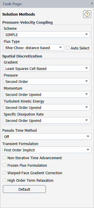
The Solution Methods task page allows you to specify various parameters associated with the solution method to be used in the calculation.
Important: This feature offers reduced functionality when running Fluent under the Pro capability level.
Controls
- Formulation
provides a drop-down list of the available types of solver formulations: Implicit and Explicit.
This item appears only when the density-based solver is used.
- Flux Type
(for the density-based solver) provides a drop-down list of the convective flux types: Roe-FDS, AUSM, and Low Diffusion Roe-FDS. Details about each of the flux types can be found in Convective Fluxes in the Theory Guide.
- Pressure-Velocity Coupling
contains settings for pressure-velocity coupling schemes.
- Scheme
(for the pressure-based solver only) provides a drop-down list of the available pressure-velocity coupling schemes: SIMPLE, SIMPLEC, PISO, and Coupled. When the non-iterative time advancement (NITA) scheme is enabled in the Solution Methods task page, Fractional Step is available for single phase flows, and Phase Coupled SIMPLE is available for Eulerian multiphase flows. See Pressure-Velocity Coupling in the Fluent Theory Guide, and Choosing the Pressure-Velocity Coupling Method, Setting Solution Controls for the Non-Iterative Solver, and Selecting the Pressure-Velocity Coupling Method for details about these methods.
- Skewness Correction
enables the SIMPLEC and PISO skewness correction for highly skewed meshes if the value (number of iterations) is greater than 0. The default value is 0 for SIMPLEC and 1 for PISO.
- Neighbor Correction
enables the PISO neighbor correction, which is recommended for transient calculations, if the value (number of iterations) is greater than 0. The default value is 1.
- Skewness-Neighbor Coupling
allows for a more economical but a less robust variation of the PISO algorithm.
- Coupled with Volume Fraction
couples velocity corrections, shared pressure corrections, and the correction for volume fraction simultaneously. This option is available in the interface after you have selected Coupled from the Scheme drop-down list for Pressure-Velocity Coupling.
- Solve N-Phase Volume Fraction Equations
solves all primary and secondary volume fraction equations and scales the resulting volume fractions to satisfy the requirement that they sum to 1. If this is disabled, only the secondary phase volume fractions are solved directly and the primary phase volume fraction is set such that the volume fractions sum to 1.
- Flux Type
(for the pressure-based solver) provides a drop-down list of the mass flux types: Rhie-Chow: distance based and Rhie-Chow: momentum based. Details about each of the flux types can be found in Discretization of the Continuity Equation in the Theory Guide. You cannot change the selection if Auto Select is enabled. For multiphase models other than the wet steam model, this list is not available and the Rhie-Chow: momentum based flux option is used.
- Auto Select
enables the automatic selection of the Flux Type, so that the most robust formulation is used for the flow models and mesh attributes of your case (for details, see Mass Flux Types). This option is enabled by default.
- Spatial Discretization
contains settings that control the spatial discretization of the convection terms in the solution equations. See Choosing the Spatial Discretization Scheme for details.
- Gradient
contains a drop-down list of the options for setting the method of computing the gradient in Equation 23–30 in the Theory Guide: Green-Gauss Cell Based; Green-Gauss Node-Based, and Least Squares Cell Based. See Evaluation of Gradients and Derivatives in the Theory Guide for details.
- Pressure
(for the pressure-based solver only) contains a drop-down list of the discretization schemes available for the pressure equation: Standard, PRESTO!, Linear, Second Order, Body Force Weighted, and Modified Body Force Weighted.
This item appears only when the pressure-based solver is used.
- Flow
(for the density-based solvers only) contains a drop-down list of the discretization schemes available for the pressure, momentum, and (if relevant) energy equations: First Order Upwind, Second Order Upwind, Third-Order MUSCL, and (if the LES, DES, SAS, SDES, or SBES turbulence model is enabled) Bounded Central Differencing.
This item appears only when one of the density-based solvers is used.
- Momentum, Energy, and so on
are the names of the other convection-diffusion equations being solved. In the drop-down list next to each equation, you can select the First Order Upwind, Second Order Upwind, QUICK, or Third-Order MUSCL discretization scheme for that equation.
If the LES, DES, SAS, SDES, or SBES turbulence model is enabled, then you have a choice of selecting Bounded Central Differencing or Central Differencing for Momentum. If Bounded Central Differencing is selected, an entry field BCD Scheme Boundedness appears under the Spatial Discretization group box.
If one of the density-based solvers is used, Momentum and Energy will not appear. For the density-based solvers, the discretization scheme for these equations is selected in the Flow drop-down list (described above).
- BCD Scheme Boundedness
specifies the boundedness strength of the BCD scheme as a constant or an expression. In the latter case, the field variable BCD Scheme Boundedness is created in the Derivatives category and can be visualized.
- Volume Fraction
is available when the VOF multiphase model is enabled. The discretization schemes that are used when solving volume fraction equations for the VOF explicit scheme are Geo-Reconstruct, Compressive, CICSAM, Modified HRIC, and QUICK. The discretization schemes that are used when solving volume fraction equations for the VOF implicit scheme are First Order Upwind, Second Order Upwind, Compressive, Modified HRIC, BGM (steady state only), and QUICK. See Interpolation Near the Interface in the Theory Guide for detailed information about these VOF-specific interpolation schemes.
- Pseudo Time Method
allows you to select a form of implicit under-relaxation (see Pseudo Time Method Under-Relaxation): the Local Time Step or Global Time Step method. This list is available for all calculations when using a pressure-based segregated solver (Local Time Step) or for steady-state calculations when using the pressure-based coupled solver or the density-based implicit solver (Global Time Step). For details on completing the setup for the pseudo time method, see Performing Calculations with a Pseudo Time Method.
- Transient Formulation
contains options for setting different time-dependent solution formulations. This option appears only when Transient is enabled under Time in the General task page. Available options include: Explicit (available only for the Density Based Explicit solver); First Order Implicit; Second Order Implicit; and Bounded Second Order Implicit. See Performing Time-Dependent Calculations for details.
- Non-Iterative Time Advancement
enables non-iterative time-advancement (NITA) scheme. See Time-Advancement Algorithm in the Theory Guide for details.
- (NITA)
Opens the NITA Options dialog box where you can enable the option and adjust the relevant controls. See Hybrid NITA for the VOF and Mixture Multiphase Models for a description of the available controls. This item is available only for the VOF and Mixture multiphase models when the Non-Iterative Time Advancement option is enabled.
- Accelerated Time Marching
enables a modified NITA scheme and other setting changes that can speed up the simulation. This option is only available with the Large Eddy Simulation (LES) turbulence model, and is intended for unreacting flow simulations that use a constant-density fluid. For details, see Setting Solution Controls for the Non-Iterative Solver.
- Frozen Flux Formulation
enables an option to discretize the convective part of Equation 23–68 in the Theory Guide using the mass flux at the cell faces from the previous time level n. This option is available only for a Transient solution. See The Frozen Flux Formulation in the Theory Guide for details.
- Warped-Face Gradient Correction
enables an adjustment to the gradient discretization method that improves the gradient accuracy for meshes containing high aspect ratios, cells with non-flat faces, and highly deformed cells, and can help avoid numerical difficulties in simulations that involve a mesh that has large differences in the volumes of neighboring cells. By default, the fast, or more computationally efficient mode of the warped-face gradient correction is used. For additional information about the warped-face gradient correction, see Warped-Face Gradient Correction.
- Convergence Acceleration For Stretched Meshes
enable convergence acceleration for stretched meshes to improve the convergence of the implicit density based solver on meshes with high cell stretching (see Convergence Acceleration for Stretched Meshes (CASM)).
- High-Speed Numerics
enables built-in, customized numeric settings that can help to stabilize and accelerate the convergence for high-speed flows. (see Enabling High-Speed Numerics).
- High Order Term Relaxation
enables the relaxation of high order terms to aid in the solution behavior of flow simulations when higher order spatial discretization is used.
opens the Relaxation Options Dialog Box.
- Turbomachinery-Specific Numerics
enables built-in customized numerics settings that can help to achieve and accelerate the convergence for turbomachinery flows. This option is only available when the Turbo Models option is enabled in the Domain ribbon tab (Turbomachinery group) for a steady calculation with the pressure-based solver selected and the Pseudo Time Method set to the Global Time Step option. For further details, see Turbomachinery-Specific Numerics.
- Set All Species Discretizations Together
enables an option to use the same discretization scheme for all the species rather than setting each of the species individually. Notice that you will no longer see your list of individual species, instead a Species field will appear with the scheme of your choice. Note that this option is available when species transport is enabled.
sets the fields to their default values, as assigned by Ansys Fluent.
- Report Poor Quality Elements
reports statistics on the number and type of cells that Ansys Fluent has identified as having poor quality.
The Relaxation Options dialog box allows you to further control the High Order Term Relaxation (HOTR), as described in High Order Term Relaxation (HOTR).
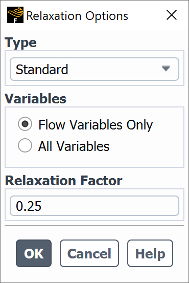
Controls
- Type
allows you to select between Standard (which is the default selection and applies HOTR to both convection and diffusion terms) or Convection Only (which applies HOTR exclusively to the convection terms). The Type list is only available with the pressure-based solver.
- Variables
allows you to select between under-relaxing All Variables or only the default flow variables (Flow Variables Only.
- Relaxation Factor
is by default 0.25 for steady-state cases and 0.75 for transient cases.