


For species transport calculations, you can model the diffusion of chemical species using the following methods:
Fickian diffusion (default)
The Fick’s law approximation is adequate for most applications. See Mass Diffusion in Laminar Flows and Mass Diffusion in Turbulent Flows in the Fluent Theory Guide for more information about the theoretical background of the mass diffusion due to concentration gradients.
Full multicomponent diffusion
For some applications (for example, diffusion-dominated laminar flows such as chemical vapor deposition), the full multicomponent diffusion model is recommended. See Full Multicomponent Diffusion in the Fluent Theory Guide for more information about the theoretical background of the full multicomponent diffusion.
Important: The full multicomponent diffusion model is enabled by selecting the Full Multicomponent Diffusion option in the Species Model Dialog Box and is computationally expensive.
By default, the solver computes the species diffusion using:
For laminar flows: Equation 7–2 in the Fluent Theory Guide
For turbulent flows: Equation 7–4 in the Fluent Theory Guide
If you have enabled the Full Multicomponent Diffusion option in the Species Model Dialog Box, then the solver computes the diffusive mass flux using Equation 7–8 in the Fluent Theory Guide.
The inputs for the diffusion coefficient for species  in the mixture (
 in Equation 7–3 in the Fluent Theory Guide) or for
the individual binary mass diffusion coefficients (
in Equation 7–3 in the Fluent Theory Guide) or for
the individual binary mass diffusion coefficients ( in Equation 7–3 or Equation 7–6 in the Fluent Theory Guide) are described in Mass Diffusion Coefficient Inputs.
To specify the mass diffusion coefficients for the mixture, follow the steps below. The diffusion coefficients have units of m2/s in SI units or ft2/s in British units.
If you are modeling full multicomponent species transport described in Full Multicomponent Diffusion in the Fluent Theory Guide, enable the Full Multicomponent Diffusion option in the Species Model Dialog Box.
If you want to account for thermal diffusion, enable the Thermal Diffusion option in the Species Model dialog box.
Open the Create/Edit Materials dialog box for the mixture material.
 Setup →
  Materials
In the Properties group box, select the specification method for the mass diffusion coefficients from the Mass Diffusivity drop-down list. The following options are available:
constant-dilute-appx: Allows you to specify a constant value for all
 in the field below. Ansys Fluent automatically uses the Fickian
diffusion (Mass Diffusion in Laminar Flows and Mass Diffusion in Turbulent Flows in the Fluent Theory Guide). This method is not available for the Full
Multicomponent Diffusion option.
in the field below. Ansys Fluent automatically uses the Fickian
diffusion (Mass Diffusion in Laminar Flows and Mass Diffusion in Turbulent Flows in the Fluent Theory Guide). This method is not available for the Full
Multicomponent Diffusion option.dilute-approx: Allows you to define each
 as a constant or as a polynomial function of temperature (if heat
transfer is enabled). Ansys Fluent automatically uses the Fickian diffusion (Mass Diffusion in Laminar Flows and Mass Diffusion in Turbulent Flows in the Fluent Theory Guide). This method is not available for the Full
Multicomponent Diffusion option.
as a constant or as a polynomial function of temperature (if heat
transfer is enabled). Ansys Fluent automatically uses the Fickian diffusion (Mass Diffusion in Laminar Flows and Mass Diffusion in Turbulent Flows in the Fluent Theory Guide). This method is not available for the Full
Multicomponent Diffusion option.See Dilute Approximation Inputs for details.
unity-lewis-number: No additional inputs are required. The mass diffusion coefficients
 are calculated under the assumption of unity Lewis number for all
species in the mixture. This method is not available for the Full
Multicomponent Diffusion option.
are calculated under the assumption of unity Lewis number for all
species in the mixture. This method is not available for the Full
Multicomponent Diffusion option.The Lewis number is the ratio of thermal diffusivity (Prandtl number) to mass diffusivity (Schmidt number). The unity-lewis-number option is a reasonable approximation when flow is highly turbulent and the contribution of laminar diffusion is small.
kinetic-theory: The solver uses kinetic theory to calculate the binary diffusion of species
 in each species
  ,
,  .
. See Multicomponent Method Inputs for details.
For the theory behind this method, see Kinetic Theory Parameters for Diffusion Coefficients in the Fluent Theory Guide.
multicomponent: Allows you to define the binary diffusion of species
in each species , as a constant or a polynomial function of temperature. See Multicomponent Method Inputs for details.
user-defined: Allows you to define a single user-defined function that applies to all mass diffusion coefficients. This is done using the
DEFINE_DIFFUSIVITYmacro and is explained in the Fluent Customization Manual.
If you are modeling a dilute mixture where the mass fraction of all species is small compared to one dominant species, choose either the constant-dilute-appx or dilute-approx method to specify
 . If you are modeling a non-dilute mixture, you may define the
individual binary mass diffusion coefficients
. If you are modeling a non-dilute mixture, you may define the
individual binary mass diffusion coefficients  . The solver will compute the diffusion of species
  in the mixture using Equation 7–3 in the Fluent Theory Guide, unless you have enabled Full Multicomponent
Diffusion the Species Model dialog box.. In the latter
case, the solver will use the inputs for the individual binary mass diffusion
coefficients
in the mixture using Equation 7–3 in the Fluent Theory Guide, unless you have enabled Full Multicomponent
Diffusion the Species Model dialog box.. In the latter
case, the solver will use the inputs for the individual binary mass diffusion
coefficients  to calculate the diffusive mass flux according to Equation 7–8 in the Fluent Theory Guide.
(turbulent flows only) Optionally, you can adjust the Turbulent Schmidt Number in the Viscous Model Dialog Box (Model Constants group box). See Mass Diffusion Coefficient Inputs for Turbulent Flow for more information.
If you have enable the Thermal Diffusion option in the Species Model dialog box, define the thermal diffusion coefficients as described in Thermal Diffusion Coefficient Inputs.
If you are modeling anisotropic species diffusion in porous media, configure appropriate settings as described in Anisotropic Species Diffusion.
To use the constant dilute approximation method, follow these steps:
Select constant-dilute-appx in the drop-down list to the right of Mass Diffusivity.
Enter a single value of
 . The same value will
be used for the diffusion coefficient of each species in the mixture.
. The same value will
be used for the diffusion coefficient of each species in the mixture.
To use the dilute approximation method, follow the steps below:
Select dilute-approx in the drop-down list to the right of Mass Diffusivity.
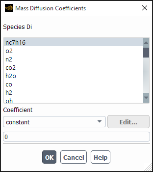
In the resulting Mass Diffusion Coefficients Dialog Box (Figure 8.34: The Mass Diffusion Coefficients Dialog Box for Dilute Approximation), select the species in the Species Di list for which you are going to define the mass diffusion coefficient.
You can define
 for the selected species either as a constant value
or (if heat transfer is active) as a polynomial function of temperature:
for the selected species either as a constant value
or (if heat transfer is active) as a polynomial function of temperature:To define a constant diffusion coefficient, select constant (the default) in the drop-down list below Coefficient, and then enter the value in the field below the list.
To define a temperature-dependent diffusion coefficient, choose polynomial in the Coefficient drop-down list and then define the polynomial coefficients as described in Inputs for Polynomial Functions.

(8–70)
Repeat steps 2 and 3 until you have defined diffusion coefficients for all species in the Species Di list in the Mass Diffusion Coefficients Dialog Box.
To use the multicomponent method, and define constant or temperature-dependent diffusion coefficients, follow the steps below:
Select multicomponent in the drop-down list to the right of Mass Diffusivity.
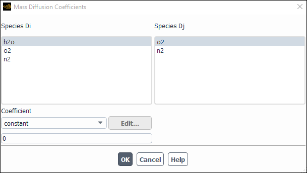
In the resulting Mass Diffusion Coefficients Dialog Box (Figure 8.35: The Mass Diffusion Coefficients Dialog Box for the Multicomponent Method), select the species in the Species Di list and the Species Dj list for which you are going to define the mass diffusion coefficient
 for species
  in species
  .
.Define
 for the selected pair of species using one of the following methods:
as a constant value or as a polynomial function of temperature (if heat transfer is
active).
for the selected pair of species using one of the following methods:
as a constant value or as a polynomial function of temperature (if heat transfer is
active).To define a constant diffusion coefficient, select constant (the default) from theCoefficient drop-down list, and then enter the value in the field below the list.
(only if heat transfer is enabled) To define a temperature-dependent diffusion coefficient, choose polynomial in the Coefficient drop-down list and then define the polynomial coefficients as described in Inputs for Polynomial Functions.

(8–71)
Repeat steps 2 and 3 until you have defined diffusion coefficients for all pairs of species in the Species Di and Species Dj lists in the Mass Diffusion Coefficients Dialog Box.
To use the multicomponent method, and define the diffusion coefficient using kinetic theory (available only when the ideal gas law is used), follow these steps:
Choose kinetic-theory in the drop-down list to the right of Mass Diffusivity.
Click after completing other property definitions for the mixture material.
Define the Lennard-Jones parameters,
 and
and  ,
for each species (fluid material), as described in Kinetic Theory Parameters.
,
for each species (fluid material), as described in Kinetic Theory Parameters.
When your flow is turbulent, you will define  or
or  , as described for laminar flows in Mass Diffusion Coefficient Inputs, and you will also have the option to alter
the default setting for the turbulent Schmidt number,
, as described for laminar flows in Mass Diffusion Coefficient Inputs, and you will also have the option to alter
the default setting for the turbulent Schmidt number,  , as defined in Equation 7–5 in the Fluent Theory Guide.
Usually, in a turbulent flow, the mass diffusion is dominated by the turbulent transport as determined by the turbulent Schmidt number (Equation 7–5 in the Fluent Theory Guide). The turbulent Schmidt number measures the relative diffusion of momentum and mass due to turbulence and is on the order of unity in all turbulent flows. Because the turbulent Schmidt number is an empirical constant that is relatively insensitive to the molecular fluid properties, you will have little reason to alter the default value (0.7) for any species.
Should you want to modify the Schmidt number, enter a new value for Turbulent Schmidt Number in the Viscous Model Dialog Box (Model Constants group box).
![]() Setup → Models → Viscous
Setup → Models → Viscous ![]() Edit...
Edit...
Important: Note that the full multicomponent diffusion model described in Full Multicomponent Diffusion in the Fluent Theory Guide is not recommended for turbulent flows.
You can model anisotropic species diffusion in porous media. For the theory behind this modeling method, see Anisotropic Species Diffusion in the Fluent Theory Guide.
To account for anisotropic species diffusion in porous media simulations:
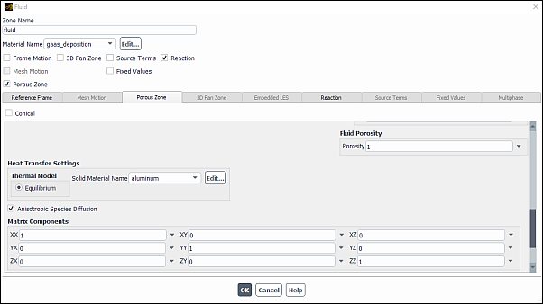
In the Fluid dialog box, enable Porous Zone.
In the Porous Zone tab, select the Anisotropic Species Diffusion check box (see Figure 8.36: Anisotropic Species Diffusion Matrix).
Specify the Matrix Components for the anisotropic diffusion matrix
 .
. If you want to include the effect of porous media tortuosity, you can modify components of the anisotropic diffusion matrix accordingly.
By default,
 is the identity matrix that corresponds to isotropic diffusion.
If you have enabled the Thermal Diffusion option in the Species Model Dialog Box, you can define the thermal diffusion coefficients in the Create/Edit Materials Dialog Box as follows:
In the Create/Edit Materials dialog box for the mixture, select one of the following methods from the Thermal Diffusion Coefficient drop-down list:
Choose kinetic-theory to have Ansys Fluent compute the thermal diffusion coefficients using the empirically-based expression in Equation 7–17 in the Fluent Theory Guide. No further inputs are required for this option.
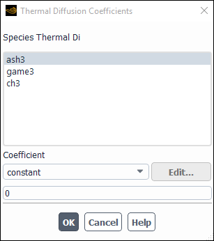
Choose specified to input the coefficient for each species in the Thermal Diffusion Coefficients Dialog Box (Figure 8.37: The Thermal Diffusion Coefficients Dialog Box) that opens automatically as further described.
Choose user-defined to use a user-defined function. More information about user-defined functions can be found in the Fluent Customization Manual.
(specified method only) For each species in the Species Thermal Di list of the Thermal Diffusion Coefficients dialog box, perform the following steps:
Select the species in the Species Thermal Di list for which you are going to define the thermal diffusion coefficient.
Define
 for the selected species either as a constant value or as a
polynomial function of temperature:
for the selected species either as a constant value or as a
polynomial function of temperature:To define a constant diffusion coefficient, select constant (the default) in the drop-down list below Coefficient, and then enter the value in the field below the list.
To define a temperature-dependent diffusion coefficient, choose polynomial in the Coefficient drop-down list and then define the polynomial coefficients as described in Defining Properties Using Temperature-Dependent Functions.
For the theory behind this method, see Thermal Diffusion Coefficients in the Fluent Theory Guide.