Under certain circumstances, it is desirable to compute not only the particle-induced wall erosion rates, but also the actual deformation of the material due to erosion. The erosion of material from the surface of the wall may create large cavities that will affect particulate flow and erosion processes and eventually lead to material failure. To account for changes in the wall's shape and position and for more accurate predictions of the erosion rates, Ansys Fluent provides the capability to couple the erosion rate solver with the dynamic mesh model.
Generally, erosion is a slow process, typically far slower than the processes on the fluid side. Ansys Fluent implements the erosion dynamic mesh model using a quasi-steady approach. During each step of the solution process, the flow and particle erosion simulations are performed as steady-state, whereas the mesh position is updated by the dynamic mesh module using the physical time step size.
When erosion is coupled with dynamic meshes, Ansys Fluent computes the mesh deformation of an
individual face  as:
as:
 | (24–13) |
| where, | |
 = Wall face specific erosion rate density = Wall face specific erosion rate density | |
 = Mesh motion time step size = Mesh motion time step size | |
 = Wall material density = Wall material density |
Before setting up a calculation of erosion coupled with the dynamic mesh model, perform the following steps:
Set up a DPM case (including defining fluid properties, setting boundary and cell zone conditions, etc.). For information on setting up a DPM calculation, see Steps for Using the Discrete Phase Models in the Fluent User's Guide.
Set up injections as described in Creating and Modifying Injections in the Fluent User's Guide.
Create report definitions to monitor flow variables.
Specify convergence criteria and solver controls for your simulation.
Initialize the flow field and run the solution.
Note that you need to compute a large number of particle trajectories in order to provide sufficiently smooth erosion patterns for the dynamic mesh motion algorithm.
Enable erosion/accretion on affected walls as described in Monitoring Erosion/Accretion of Particles at Walls and Setting Particle Erosion and Accretion Parameters in the Fluent User's Guide.
Once erosion/accretion is enabled, the Erosion Dynamic Mesh item appears in the tree under the Setup/Models/Discrete Phase tree branch.
Perform a calculation for the erosion rates.
Note: Note that it is not necessary to initialize the flow field and calculate both flow and erosion prior to coupling erosion with dynamic mesh. However, it will speed up the erosion dynamic mesh simulation if you start from a converged flow field and then follow with a first estimation of the erosion rates.
Once the solution is completed, select Steady in the Genteral task page (Solver group).
Note the following limitations when modeling wall erosion coupled with the dynamic mesh model:
Erosion coupling with dynamic mesh is available only for steady-state flows due to being implemented via a quasi-steady approach.
You can run the erosion dynamic mesh simulation via either the Erosion Dynamic Mesh Coupling Setup dialog box or the
define/models/dpm/erosion-dynamic-mesh/run-simulationtext command, but not from the Run Calculation task page or via thesolve/iteratetext command.
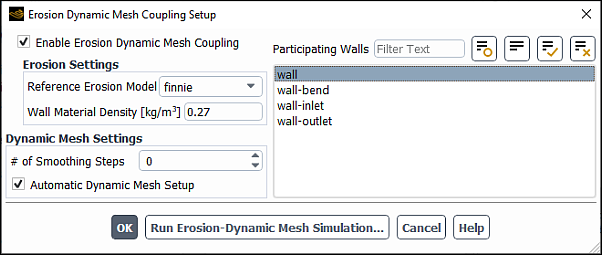
Open the Erosion Dynamic Mesh Coupling Setup dialog box and select Enable Erosion Dynamic Mesh Coupling.
 Setup → Models
→ Discrete Phase → Erosion Dynamic
Mesh
Setup → Models
→ Discrete Phase → Erosion Dynamic
Mesh  Edit...
In the Erosion Settings group box, select an appropriate Reference Erosion Model for your simulation and specify the Wall Material Density.
You can choose from the following erosion models:
finnie (default)
generic-model
mclaury
oka
dnv
For information about these models, refer to Setting Particle Erosion and Accretion Parameters in the Fluent User's Guide.
Note that these models will not be available if you are using a UDF to specify the erosion accretion rates as described in
DEFINE_DPM_EROSIONin the Fluent Customization Manual. In this case, only udf will appear in Reference Erosion Model.The wall material density is assumed to be identical for all walls involved in the erosion coupled with dynamic mesh simulation. Note that for Wall Material Density, you may need to adjust the default value of 2719 kg/m3, which is the density of aluminum.
(dense flows with the disperse granular phase only) If you want to model abrasive erosion rates and wall shielding effects, select Include Abrasive Erosion Effects. For more information about these models, refer to Modeling Erosion Rates in Dense Flows in the Fluent Theory Guide.
In the Dynamic Mesh Settings group box, you can:
Specify a non-zero value for # of Smoothing Steps if you want to apply smoothing to the wall erosion rates in the dynamic mesh module.
Smoothing the erosion rates is recommended. For cases with a lower particle count, you can increase the # of Smoothing Steps to a value greater than 1. Note that tracking a sufficient number of particles in your simulation will ensure no large variations in erosion rate density. If you refine your mesh by a factor of 2 in each direction, you also need to increase the number of particles by a factor of 4 or more.
Enable Automatic Dynamic Mesh Setup (default)
The Automatic Dynamic Mesh Setup allows for a quick setup of the basic functionalities needed for an erosion dynamic mesh coupled simulation. Selecting this option automatically enables Dynamic Mesh and the smoothing and remeshing methods. These methods will ensure that the mesh quality remains acceptable during the simulation. The option also automatically creates a dynamic zone of a User-Defined type for each zone participating in the coupled erosion dynamic mesh simulation. The motion of the dynamic zones is defined by the **erosion** mesh motion UDF provided by Ansys Fluent.
For additional information, see the following sections:
The automatic dynamic mesh setup uses the dynamic mesh methods with reasonable defaults, which may not be optimal for all cases. If you want to modify the dynamic mesh settings after the automatic setup has been completed, you must first disable Automatic Dynamic Mesh Setup; otherwise, your changes will be overwritten by the default settings. Before adjusting the dynamic mesh settings, you should become familiar with the Deform Adjacent Boundary Layer with Zone and Feature Detection options, which are described in Boundary Layer Smoothing Method and Feature Detection in the Fluent User's Guide. Note that if you are setting up erosion / accretion on a moving wall between a fluid and solid zone, you must create a deforming zone for the solid zone that uses the radial basis function smoothing method (for details, see Radial Basis Function Smoothing).
From the Participating Walls selection list, select walls that will be deformed due to particle-wall erosion. Note that if you are setting up erosion / accretion between a fluid and solid zone, the fluid side of the coupled wall should be selected under Participating Walls, not the solid side.
To set controls for the erosion dynamic mesh solver and then run the simulation, click Run Erosion-Dynamic Mesh Simulation….
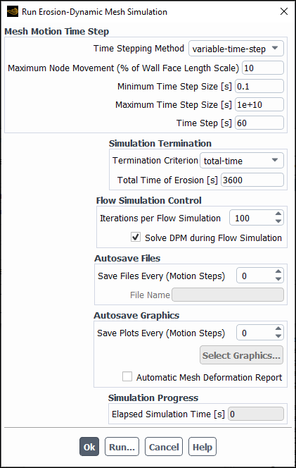
In the Mesh Motion Time Setup group box, you can select the time stepping method to compute the mesh deformation from Equation 24–13:
fixed-time-step: allows you to specify a constant Time Step.
variable-time-step (default): is automatically determined by the dynamic mesh solver based on the following parameters:
- Maximum Node Movement (% of Wall Face Length Scale)
the maximum allowed cell deformation per meshing step. It is specified as a fraction (in percent) of the characteristic length, which is derived from the cell wall face area. A default of 10% is an acceptable, conservative value. To speed up the calculation, you can set this parameter to a higher value. A value of 20 to 30%, or even higher, is suitable in most cases. However, because the erosion rate is considered to be constant during each time step, some erosion rate variations may be lost for larger mesh deformations. Trial and error may be required to find an optimal value for your case input.
- Minimum/Maximum Time Step Size
upper and lower time limits. If you want the solver to use the time step calculated by the dynamic mesh module, set Maximum Time Step Size to a large value.
During the iteration process, the solver adjusts the time step based on the maximum node movement. The solver will gradually increase the time step up to its maximum value, resulting in a faster overall simulation time. Ansys Fluent will report the time step used in the current iteration in the console and in the Time Step field.
In the Simulation Termination group box, specify the Total Time of Erosion (in seconds). The simulation stops when the specified time period ends.
In the Flow Simulation Control group box, you can specify:
Iterations per Flow Simulation: is the number of flow iterations between mesh deformation steps. This number should be sufficiently large to ensure that the flow simulation converges between successive mesh steps.
(only when Interaction with Continuous Phase is enabled) Solve DPM during Flow Simulation: enforces a tighter coupling between gas and particle phases. During the flow calculation, the particle tracker will be called regularly at the frequency specified in DPM Iteration Interval in the Discrete Phase Model dialog box.
If you want to automatically save case and data files during the calculation, you can specify a filename and a frequency with which case and data files should be saved for postprocessing or restart purposes in the Autosave Files group box. When saving case and data files, Ansys Fluent appends the filename that you have provided with
@time=.flow timeSpecify the autosave plot options in the Autosave Graphics group box.
If you want to capture images of mesh, contour, or vector plots at the specified intervals for later use (for example, to generate animations of your solution over time), set the frequency at which your plots will be saved in the Save Plots Every text entry field and click .
Note: The Select Graphics... button becomes available only after the flow field has been initialized.
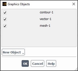
In the Graphics Objects dialog box, from the New Object drop-down list, select the object that you want to save:
Mesh... opens the Mesh Display Dialog Box
Contours... opens the Contours Dialog Box
Vectors... opens the Vectors Dialog Box
Once you create a new object, it will be displayed in the Graphics Objects dialog box.
Select which graphics objects you want to save as PNG images during the solution run. Similar to case and data files, the image filenames will be appended with
@time=.flow time
If you want Ansys Fluent to plot the vertex maximum of the accumulated deformation variable on all walls undergoing mesh deformation, enable Automatic Mesh Deformation Report.
When you start iterating, Ansys Fluent automatically creates the max-accumulated-deformation report definition and max-accumulated-deformation-pset report plot, which will be displayed in the graphics window during the solution run.
Click Run... in the Run Erosion-Dynamic Mesh Simulation dialog box.
Important: The erosion dynamic mesh simulation must be run only from the Run Erosion-Dynamic Mesh Simulation dialog box.
During the coupled erosion dynamic mesh analysis, first, the erosion module computes erosion rates and passes them to the dynamic mesh module. The dynamic mesh module performs a pseudo-steady simulation of the mesh deformation. After that, the solver carries out a steady-state flow calculation for a specified number of flow iterations. If Solve DPM during Flow Simulation is enabled, the particle tracking is performed in the specified DPM Iteration Interval. Otherwise, the particle tracker is run once after the flow calculation is finished. Whenever the particle tracker is run, the DPM sources are updated. This process is repeated until the specified Total Time Of Erosion is reached.
As the solution progresses, Ansys Fluent reports the dynamic mesh time step and the simulation time in the console and the Time Step and Elapsed Simulation Time fields. If you interrupt the simulation using the Interrupt Simulation dialog box, the solver will complete the current flow and erosion iterations before stopping the calculation.