


Compressibility effects are encountered in gas flows at high velocity and/or in which there
are large pressure variations. When the flow velocity approaches or exceeds the speed of
sound of the gas or when the pressure change in the system ( ) is large, the variation of the gas density with pressure has a
significant impact on the flow velocity, pressure, and temperature. Compressible flows
create a unique set of flow physics for which you must be aware of the special input
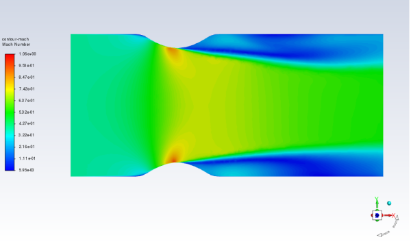
requirements and solution techniques described in this section. Figure 9.12: Flow in a Converging-Diverging Nozzle shows compressible flows computed using
Ansys Fluent.
) is large, the variation of the gas density with pressure has a
significant impact on the flow velocity, pressure, and temperature. Compressible flows
create a unique set of flow physics for which you must be aware of the special input
requirements and solution techniques described in this section. Figure 9.12: Flow in a Converging-Diverging Nozzle shows compressible flows computed using
Ansys Fluent.
Information about compressible flows is provided in the following subsections:
For more information about the theoretical background of compressible flows, see Compressible Flows in the Theory Guide.
Compressible flows can be characterized by the value of the Mach number:
 | (9–16) |
Here,  is the speed of sound in the gas:
 | (9–17) |
and  is the ratio of specific heats
  .
.
When the Mach number is less than 1.0, the flow is termed subsonic.
At Mach numbers much less than 1.0 ( or so), compressibility effects are negligible and
the variation of the gas density with pressure can safely be ignored
in your flow modeling. As the Mach number approaches 1.0 (which is
referred to as the transonic flow regime), compressibility effects
become important. When the Mach number exceeds 1.0, the flow is termed
supersonic, and may contain shocks and expansion fans which can impact
the flow pattern significantly. Ansys Fluent provides a wide range of
compressible flow modeling capabilities for subsonic, transonic, and
supersonic flows.
or so), compressibility effects are negligible and
the variation of the gas density with pressure can safely be ignored
in your flow modeling. As the Mach number approaches 1.0 (which is
referred to as the transonic flow regime), compressibility effects
become important. When the Mach number exceeds 1.0, the flow is termed
supersonic, and may contain shocks and expansion fans which can impact
the flow pattern significantly. Ansys Fluent provides a wide range of
compressible flow modeling capabilities for subsonic, transonic, and
supersonic flows.
Compressible flows are typically characterized by the total
pressure  and total
temperature
and total
temperature  of the flow.
For an ideal gas, these quantities can be related to the static pressure
and temperature by the following:
of the flow.
For an ideal gas, these quantities can be related to the static pressure
and temperature by the following:
 | (9–18) |
For constant  , Equation 9–18 reduces to
 | (9–19) |
These relationships describe the variation of the static pressure
and temperature in the flow as the velocity (Mach number) changes
under isentropic conditions. For example, given a pressure ratio from
inlet to exit (total to static), Equation 9–19 can
be used to estimate the exit Mach number that would exist in a one-dimensional
isentropic flow. For air, Equation 9–19  ,
of 0.5283. This choked flow condition will be established at the point
of minimum flow area (for example, in the throat of a nozzle). In
the subsequent area expansion the flow may either accelerate to a
supersonic flow in which the pressure will continue to drop, or return
to subsonic flow conditions, decelerating with a pressure rise. If
a supersonic flow is exposed to an imposed pressure increase, a shock
will occur, with a sudden pressure rise and deceleration accomplished
across the shock.
,
of 0.5283. This choked flow condition will be established at the point
of minimum flow area (for example, in the throat of a nozzle). In
the subsequent area expansion the flow may either accelerate to a
supersonic flow in which the pressure will continue to drop, or return
to subsonic flow conditions, decelerating with a pressure rise. If
a supersonic flow is exposed to an imposed pressure increase, a shock
will occur, with a sudden pressure rise and deceleration accomplished
across the shock.
Compressible flows are described by the standard continuity and momentum equations solved by Ansys Fluent, and you do not need to enable any special physical models (other than the compressible treatment of density as detailed below). The energy equation solved by Ansys Fluent correctly incorporates the coupling between the flow velocity and the static temperature, and should be activated whenever you are solving a compressible flow. In addition, if you are using the pressure-based solver, you should enable the viscous dissipation terms in Equation 5–1 in the Theory Guide, which become important in high-Mach-number flows.
For compressible flows, the ideal gas law is written in the following form:
 | (9–20) |
where  is the operating
pressure defined in the Operating Conditions Dialog Box,
is the operating
pressure defined in the Operating Conditions Dialog Box,  is the local static pressure relative to the operating
pressure,
is the local static pressure relative to the operating
pressure,  is the universal gas constant, and
  is the molecular
weight. The temperature,
is the molecular
weight. The temperature,  , will be computed from the energy equation.
Some compressible flow problems involve fluids that do not behave as ideal gases. For example, flow under very high-pressure conditions cannot typically be modeled accurately using the ideal-gas assumption. Therefore, the real gas model described in Real Gas Models should be used instead.
To set up a compressible flow in Ansys Fluent, you must follow the steps listed below. (Only those steps relevant specifically to the setup of compressible flows are listed here. You must set up the rest of the problem as usual.)
Set the Operating Pressure in the Operating Conditions Dialog Box.
 Setup →
  Boundary Conditions → Operating Conditions...
(You can think of
 as the absolute
static pressure at a point in the flow where you will define the gauge
pressure
as the absolute
static pressure at a point in the flow where you will define the gauge
pressure  to be zero. See Operating Pressure for guidelines on setting the operating pressure. For time-dependent
compressible flows, you may want to specify a floating operating pressure
instead of a constant operating pressure. See Floating Operating Pressure for details.)
to be zero. See Operating Pressure for guidelines on setting the operating pressure. For time-dependent
compressible flows, you may want to specify a floating operating pressure
instead of a constant operating pressure. See Floating Operating Pressure for details.)Enable the solution of the energy equation.
Setup → Models → Energy On
On
(Pressure-based solver only) If you are modeling turbulent flow, enable the optional viscous dissipation terms in the energy equation by turning on Viscous Heating in the Viscous Model Dialog Box. Note that these terms can be important in high-speed flows.
Setup → Models →  Viscous → Edit...
This step is not necessary if you are using one of the density-based solvers, because the density-based solvers always include the viscous dissipation terms in the energy equation.
Set the following items in the Create/Edit Materials Dialog Box:
Setup → Materials → Create/Edit...
Select ideal-gas in the drop-down list next to Density.
Define all relevant properties (specific heat, molecular weight, thermal conductivity, and so on).
Set cell zone conditions and boundary conditions (using the Boundary Conditions Task Page and Cell Zone Conditions Task Page), being sure to choose a well-posed cell zone or boundary condition combination that is appropriate for the flow regime. See below for details. Recall that all inputs for pressure (either total pressure or static pressure) must be relative to the operating pressure, and the temperature inputs at inlets should be total (stagnation) temperatures, not static temperatures.
Setup → Cell Zone Conditions Setup → Boundary Conditions
These inputs should ensure a well-posed compressible flow problem. You will also want to consider special solution parameter settings, as noted in Solution Strategies for Compressible Flows, before beginning the flow calculation.
Well-posed inlet and exit boundary conditions for compressible flow are listed below:
For flow inlets:
Pressure inlet: Inlet total temperature and total pressure and, for supersonic inlets, static pressure
Mass-flow inlet: Inlet mass flow and total temperature
For flow exits:
Pressure outlet: Exit static pressure (ignored if flow is supersonic at the exit. All the information travels downstream in a supersonic region, hence the pressure at the outlet can be computed by directly extrapolating from the adjacent cell center [64]. Therefore, it is not meaningful to use the exit static pressure prescribed in the boundary conditions task page, and the exit static pressure is ignored).
Mass-flow outlet: Outlet mass flow
It is important to note that your boundary condition inputs for pressure (either total pressure or static pressure) must be in terms of gauge pressure — that is, pressure relative to the operating pressure defined in the Operating Conditions Dialog Box, as described above.
All temperature inputs at inlets should be total (stagnation) temperatures, not static temperatures.
Ansys Fluent provides a “floating operating pressure” option to handle time-dependent compressible flows with a gradual increase in the absolute pressure in the domain. This option is desirable for slow subsonic flows with static pressure build-up, since it efficiently accounts for the slow changing of absolute pressure without using acoustic waves as the transport mechanism for the pressure build-up.
Examples of typical applications include the following:
combustion or heating of a gas in a closed domain
pumping of a gas into a closed domain
The floating operating pressure option should not be used for transonic or incompressible flows. In addition, it cannot be used if your model includes any pressure inlet, pressure outlet, exhaust fan, inlet vent, intake fan, outlet vent, or pressure far field boundaries.
The floating operating pressure option allows Ansys Fluent to calculate the pressure rise (or drop) from the integral mass balance, separately from the solution of the pressure correction equation. When this option is activated, the absolute pressure at each iteration can be expressed as
 | (9–21) |
where  is the pressure relative to the reference location,
which in this case is in the cell with the minimum pressure value.
Therefore the reference location itself is floating.
is the pressure relative to the reference location,
which in this case is in the cell with the minimum pressure value.
Therefore the reference location itself is floating.
 is referred to as the floating
operating pressure, and is defined as
is referred to as the floating
operating pressure, and is defined as
 | (9–22) |
where  is the initial operating pressure and
  is the pressure rise.
Including the pressure rise  in the floating operating pressure
  , rather than
in the pressure
, rather than
in the pressure  , helps to prevent roundoff error. If the pressure
rise were included in
, helps to prevent roundoff error. If the pressure
rise were included in  , the calculation of the pressure gradient for the
momentum equation would give an inexact balance due to precision limits
for 32-bit real numbers.
, the calculation of the pressure gradient for the
momentum equation would give an inexact balance due to precision limits
for 32-bit real numbers.
When time dependence is active, you can turn on the Floating Operating Pressure option in the Operating Conditions Dialog Box.
![]() Setup →
Setup → ![]() Boundary Conditions → Operating Conditions...
Boundary Conditions → Operating Conditions...
(Note that the inputs for Reference Pressure Location will disappear when you enable Floating Operating Pressure, since these inputs are no longer relevant.)
Important: The floating operating pressure option should not be used for transonic flows or for incompressible flows. It is meaningful only for slow subsonic flows of ideal or real gases, when the characteristic time scale is much larger than the sonic time scale.
When the floating operating pressure option is enabled, you must specify a value for the Initial Operating Pressure in the Solution Initialization Task Page.
![]() Solution →
Solution → ![]() Initialization
Initialization
This initial value is stored in the case file with all your other initial values.
The current value of the floating operating pressure is stored in the data file. If you visit the Operating Conditions Dialog Box after a number of time steps have been performed, the current value of the Operating Pressure will be displayed.
Note that the floating operating pressure will automatically be reset to the initial operating pressure if you reset the data (that is, start over at the first iteration of the first time step).
You can monitor the absolute pressure during the calculation using the Surface Report Definition Dialog Box. You can also generate graphical plots or alphanumeric reports of absolute pressure when your solution is complete. The Absolute Pressure variable is contained in the Pressure... category of the variable selection drop-down list that appears in postprocessing dialog boxes. See Field Function Definitions for its definition.
The difficulties associated with solving compressible flows are a result of the high degree of coupling between the flow velocity, density, pressure, and energy. This coupling may lead to instabilities in the solution process and, therefore, may require special solution techniques in order to obtain a converged solution. In addition, the presence of shocks (discontinuities) in the flow introduces an additional stability problem during the calculation. Solution techniques that may be beneficial in compressible flow calculations include the following:
(Pressure-based solver only) Initialize the flow to be near stagnation (that is velocity small but not zero, pressure to inlet total pressure, temperature to inlet total temperature). Turn off the energy equation for the first 50 iterations. Leave the energy under-relaxation at 1. Set the pressure under-relaxation to 0.4, and the momentum under-relaxation to 0.3. After the solution stabilizes and the energy equation has been turned on, increase the pressure under-relaxation to 0.7.
Set reasonable limits for the temperature and pressure (in the Solution Limits Dialog Box) to avoid solution divergence, especially at the start of the calculation. If Ansys Fluent prints messages about temperature or pressure being limited as the solution nears convergence, the high or low computed values may be physical, and you must change the limits to allow these values.
If required, begin the calculations using a reduced pressure ratio at the boundaries, increasing the pressure ratio gradually in order to reach the final desired operating condition. If the Mach number is low, you can also consider starting the compressible flow calculation from an incompressible flow solution (although the incompressible flow solution can in some cases be a rather poor initial guess for the compressible calculation).
In some cases, computing an inviscid solution as a starting point may be helpful.
See Using the Solver for details on the procedures used to make these changes to the solution parameters.
You can display the results of your compressible flow calculations in the same manner that you would use for an incompressible flow. The variables listed below are of particular interest when you model compressible flow:
Total Temperature
Total Pressure
Mach Number
These variables are contained in the variable selection drop-down list that appears in postprocessing dialog boxes. Total Temperature is in the Temperature... category, Total Pressure is in the Pressure... category, and Mach Number is in the Velocity... category. See Field Function Definitions for their definitions.