Some engineering problems involve fluids that do not behave as ideal gases. For example, at very high-pressure or very low-temperature conditions (for example, the flow of a refrigerant through a compressor) the flow cannot typically be modeled accurately using the ideal-gas assumption. Therefore, the real gas model allows you to solve accurately for the fluid flow and heat transfer problems where the working fluid behavior deviates from the ideal-gas assumption.
Ansys Fluent provides three real gas options for solving these types of flows:
All the models allow you to solve for either a single-species fluid flow or a multiple-species mixture fluid flow.
In addition, real gas property (RGP) table files can be used to incorporate material properties from external sources into an Ansys Fluent simulation.
For additional information, see the following sections:
The states at which a pure material can exist can be graphically represented in diagrams of pressure vs. temperature (PT diagrams) and pressure vs. molecular or specific volume (PV diagrams). Homogeneous fluids are normally divided into two classes, liquids and gases. However the distinction cannot always be sharply drawn, because the two phases become indistinguishable at what is called the critical point. A typical pressure-temperature (PT) diagram of a pure material is shown in Figure 8.39: Typical PT Diagram of a Pure Material.
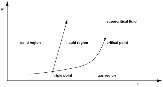
This figure shows the single phase regions, as well as the conditions
of P and T where two phases coexist. Therefore the solid and the gas
region are divided by the sublimation curve, the liquid and gas regions
by the vaporization curve, and the solid and liquid regions by the
fusion curve. The three curves meet at the triple point, where all
three phases coexist in equilibrium. Although the fusion curve continues
upward indefinitely, the vaporization curve terminates at the critical
point. The coordinates of this point are called the critical pressure  and critical
temperature
and critical
temperature  . These represent the highest
temperature and pressure at which a pure material can exist in vapor-liquid
equilibrium. At temperatures and pressures above the critical point,
the physical property differences that differentiate the liquid phase
from the gas phase become less defined. This reflects the fact that,
at extremely high temperatures and pressures, the liquid and gaseous
phases become indistinguishable. This new phase, which has some properties
that are similar to a liquid and some properties that are similar
to a gas, is called a supercritical fluid.
. These represent the highest
temperature and pressure at which a pure material can exist in vapor-liquid
equilibrium. At temperatures and pressures above the critical point,
the physical property differences that differentiate the liquid phase
from the gas phase become less defined. This reflects the fact that,
at extremely high temperatures and pressures, the liquid and gaseous
phases become indistinguishable. This new phase, which has some properties
that are similar to a liquid and some properties that are similar
to a gas, is called a supercritical fluid.
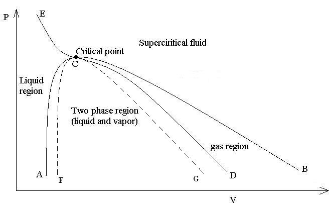
Figure 8.40: Typical PV Diagram of a Pure Material presents a typical
diagram of pressure versus molar or specific volume (PV diagram) of
a pure material. The dome shaped curve ACD is called the saturation
dome and separates the single phase regions in the diagram; curve
AC represents the saturated liquid and curve CD the saturated vapor.
The area under the saturation dome ACD is the two-phase region and
represents all possible mixtures of vapor and liquid in equilibrium.
Curve ECB is the critical isotherm and exhibits a horizontal inflection
at point C at the top of the dome. This is the critical point. The
specific volume corresponding to the critical point, is called the
critical specific volume  . The conditions to the right
of the critical isotherm ECB correspond to supercritical fluid. The
dashed lines CF and CG in Figure 8.40: Typical PV Diagram of a Pure Material represent the liquid and the vapor spinodal curves with the regions
ACF and DCG between the saturation and spinodal lines representing
the superheated liquid and supercooled vapor states, respectively.
These states are called "metastable" because they exist temporarily
in small local regions until phase change occurs. As an example, liquid
metastable states may be formed in situations of fast depressurization,
depending on the rate of depressurization and the disturbances that
tend to make the liquid flash into vapor.
. The conditions to the right
of the critical isotherm ECB correspond to supercritical fluid. The
dashed lines CF and CG in Figure 8.40: Typical PV Diagram of a Pure Material represent the liquid and the vapor spinodal curves with the regions
ACF and DCG between the saturation and spinodal lines representing
the superheated liquid and supercooled vapor states, respectively.
These states are called "metastable" because they exist temporarily
in small local regions until phase change occurs. As an example, liquid
metastable states may be formed in situations of fast depressurization,
depending on the rate of depressurization and the disturbances that
tend to make the liquid flash into vapor.
The equation of state is the mathematical expression that relates pressure, molar or specific volume, and temperature for any pure homogeneous fluid in equilibrium states.
The simplest equation of state is the ideal gas law, which is approximately valid for the low pressure gas region of the PT and PV diagrams. Ideal gas behavior can be expected when

or
 and
and 
If your flow conditions correspond to either of those cases, you may use the ideal gas law in your simulation.
Another idealization, that of the incompressible fluid, can be employed for the low pressure region of the liquid phase. A constant density option is the appropriate selection in that case.
However, both of these approaches are not good approximations for flow conditions close to and beyond the critical point, where the fluid behavior cannot be described by the ideal gas, or the incompressible liquid assumptions. We refer to a fluid under those conditions as a real fluid, or a real gas and more complex relations are used for the determination of its physical and thermodynamic properties.
Ansys Fluent provides the following options for solving real fluid problems:
The cubic equation of state models can be used to solve problems in the gas, liquid, and supercritical fluid regimes. The models are not available for the two-phase region under the phase dome. For further details see Cubic Equation of State Models.
The NIST real gas model can be used to solve problems in the liquid, or gas and supercritical fluid regimes. The model does not allow modeling of the two-phase region. For further details see The NIST Real Gas Models.
The user-defined real gas model allows you to solve problems in all regimes, as long as appropriate relationships are provided through the user-defined real gas functions. For further details see The User-Defined Real Gas Model.
The concepts presented in this section for pure materials are also extended to multicomponent mixtures with the introduction of appropriate composition-dependent parameters in the real gas equations of state and the material property models. All the real-gas modeling options above allow for either single-species or multicomponent flow modeling. In addition, you may solve reacting flow problems with the cubic equations of state models and the user-defined real gas functions.
An equation of state is a thermodynamic equation, which provides a mathematical relationship between two or more state functions associated with the matter, such as its temperature, pressure, volume, or internal energy. One of the simplest equations of state for this purpose is the ideal gas law, which is roughly accurate for gases at low pressures and high temperatures. However, this equation becomes increasingly inaccurate at higher pressures and lower temperatures, and fails to predict condensation from a gas to a liquid.
Introduced in 1949, the Redlich-Kwong equation of state [122] was a considerable improvement over other equations of that time. It is an analytic cubic equation of state and is still of interest primarily due to its relatively simple form. The original form is
 | (8–75) |
| where | |
| P = absolute pressure (Pa) | |
| R = universal gas constant | |
V = specific molar volume ( ) ) | |
| T = temperature (K) | |
 = reduced temperature = reduced temperature  , where , where  is the critical
temperature is the critical
temperature | |
 and and  are constants related directly to the fluid critical
pressure and temperature are constants related directly to the fluid critical
pressure and temperature |
Many investigators have attempted to improve the accuracy of the Redlich-Kwong equation. Ansys Fluent has adopted the original form of the Redlich-Kwong equation, as well as the following modified forms:
The Soave-Redlich-Kwong [152] equation is a three-parameter equation of state, which can be applied for vapor, supercritical, and liquid property predictions. It has found wide acceptance mainly in the oil and gas industry and requires knowledge of the critical temperature, critical pressure, and acentric factor. It was developed by replacing the Redlich-Kwong attractive coefficient defined as
 with a two-parameter form
  , where
  is the acentric factor.
The Peng-Robinson equation [117] is a three-parameter equation of state, also requiring the critical temperature, critical pressure and acentric factor parameters. It is thought to perform as well as the Soave-Redlich-Kwong equation, with an advantage in the prediction of the liquid densities.
The Aungier-Redlich-Kwong [15] equation provides improved predictions for vapor and supercritical fluids near the critical point, as well as for materials with a negative value of the acentric factor. The Aungier modified form is a four parameter equation and requires the critical specific volume in addition to the critical temperature, critical pressure and acentric factor.
The following limitations exist in Ansys Fluent for all cubic equation of state models:
Pressure-inlets, mass flow-inlets, and pressure-outlets are the only inflow and outflow boundaries available for use with the real gas models.
Non-reflecting boundary conditions are not compatible with the real gas models when using the density-based solver. If your model requires NRBC and a real gas model, you must use the pressure-based solver.
The cubic equation of state real gas models are compatible with the Eulerian multiphase models.
The cubic equation of state models are compatible with the Lagrangian Dispersed Phase Models. If you are modeling droplet or multicomponent particles, note that the current formulation does not take into account the near-critical point phenomena, which means that accurate results can be obtained for droplet temperatures below
 . See Using the Cubic Equation of State Models with the Lagrangian
Dispersed Phase Models for
more details.
. See Using the Cubic Equation of State Models with the Lagrangian
Dispersed Phase Models for
more details.The real gas models are not available with the premixed, inert, and composition PDF transport combustion models.
The cubic equation of state real gas models can be used with the following species models:
Species transport. Chemical reactions can be modeled with the finite rate and eddy dissipation models. Note that the Dimension Reduction model is not available with the real gas models.
Non-premixed model and partially-premixed model. Note that the Compressibility Effects option must be enabled in the Species Model dialog box in order for the real-gas models to be available. In addition the following restrictions apply when the non-premixed model is used together with a cubic equation of state real-gas model:
The empirical stream options cannot be used, as for the empirical species the critical properties cannot be defined.
Condensed species such as h2o<l> and c<s> are not supported and should be excluded from the PDF table, so ensure that you add all condensed species for your system in the excluded species list prior to the PDF table generation.
The laminar flame speeds for the partially-premixed model are assumed to be the same as for ideal-gases.
When the cubic equation of state models are applied for subcritical conditions near or under the phase dome, the two-phase flow is not modeled and either vapor or liquid state must be selected. Subcritical and supercritical states can co-exist in the same simulation.
The general form of pressure P for the cubic equation of state models is written as [15] :
 | (8–76) |
| where | |
|
P = absolute pressure (Pa) | |
|
V = specific molar volume ( | |
|
T = temperature (K) | |
|
R = universal gas constant |

The coefficients  ,
,  ,
,  ,
,  , and
, and  are
given for each equation of state as functions of the critical temperature
are
given for each equation of state as functions of the critical temperature  , critical pressure
  , acentric factor
  and critical specific volume
  . Note that the attractive coefficient
  also has a temperature
dependence, which varies for each equation of state model, and is
commonly written as
also has a temperature
dependence, which varies for each equation of state model, and is
commonly written as  .
.
Redlich-Kwong Equation [128]:
 | (8–77) |
 | (8–78) |
 | (8–79) |
The parameter  is set equal to
  , while
  and
and  are set to 0. The Redlich-Kwong
equation is the simplest of the cubic equations of state in Ansys Fluent and
requires two parameters only, the critical temperature
are set to 0. The Redlich-Kwong
equation is the simplest of the cubic equations of state in Ansys Fluent and
requires two parameters only, the critical temperature  and the critical pressure
  .
.
Soave-Redlich-Kwong Equation [152]:
 | (8–80) |
 | (8–81) |
 and
and  are given by Equation 8–78 and Equation 8–79 respectively. As in the original Redlich-Kwong
equation the parameter
are given by Equation 8–78 and Equation 8–79 respectively. As in the original Redlich-Kwong
equation the parameter  is set equal to
  , while
  and
and  are set to 0. The Soave-Redlich-Kwong
requires three parameters, the critical temperature
are set to 0. The Soave-Redlich-Kwong
requires three parameters, the critical temperature  , the critical pressure
  , and the acentric factor
  .
.
Peng-Robinson Equation [117]:
 | (8–82) |
 | (8–83) |
The function  is given by Equation 8–80,
with n provided in Equation 8–84 as follows:
is given by Equation 8–80,
with n provided in Equation 8–84 as follows:
 | (8–84) |
In the Peng-Robinson equation  is set equal to
  ,
,  is equal to
  , and
, and  is set to 0.
Similar to the Soave-Redlich-Kwong equation, the Peng-Robinson
equation is a three-parameter equation and requires the critical temperature  , the critical pressure
  , and the acentric factor
  .
.
Aungier-Redlich-Kwong Equation [15]:
 | (8–85) |
 | (8–86) |
 and
and  are given by Equation 8–78 and Equation 8–79, respectively. As in the original Redlich-Kwong
equation, the parameter
are given by Equation 8–78 and Equation 8–79, respectively. As in the original Redlich-Kwong
equation, the parameter  is set equal to
  and
and  is set to 0. Parameter
  is given by:
 | (8–87) |
The Aungier-Redlich-Kwong equation requires four parameters,
namely the critical temperature  , the critical pressure
  , the critical specific volume
  , and the acentric factor
  .
.
Enthalpy, entropy, and specific heat are computed in terms of
the relevant ideal gas properties and the departure functions. The
departure function  of
any conceptual property
of
any conceptual property  is defined as [122]
 | (8–88) |
where  is the value of the property as computed
from the ideal gas relations. The departure function
is the value of the property as computed
from the ideal gas relations. The departure function  can be derived from basic thermodynamic relations
and the equation of state.
can be derived from basic thermodynamic relations
and the equation of state.
Following the above definition, the enthalpy  for the equations of state
models is given by the following equations [15]:
for the equations of state
models is given by the following equations [15]:
 | (8–89) |
 | (8–90) |
 | (8–91) |
| where, | |
 = ideal gas enthalpy at temperature T (J/kg) = ideal gas enthalpy at temperature T (J/kg) | |
 =
departure enthalpy (J/kmol) =
departure enthalpy (J/kmol) | |
 = mean molecular weight (Kg/kmol) = mean molecular weight (Kg/kmol) | |
 = pressure (Pa) = pressure (Pa) | |
 = specific molar volume ( = specific molar volume ( /kmol) /kmol) | |
 = universal gas constant = universal gas constant | |
 , ,  , and , and  are computed using Equation 8–77– Equation 8–87 depending on the equation of state model are computed using Equation 8–77– Equation 8–87 depending on the equation of state model |
See Equation 8–76 for a description of other coefficients.
Similarly, the departure internal energy  can
be shown to be
can
be shown to be
 | (8–92) |
| where | |
 =
departure internal energy (J/kmol) =
departure internal energy (J/kmol) | |
 = temperature (K) = temperature (K) | |
 = specific molar volume
( = specific molar volume
( /kmol) /kmol) | |
 is given by Equation 8–91 is given by Equation 8–91
| |
 , ,  , and , and  are computed using Equation 8–77 – Equation 8–87 depending on the equation of state model are computed using Equation 8–77 – Equation 8–87 depending on the equation of state model |
The specific heat  can be computed from the ideal
specific heat
can be computed from the ideal
specific heat  and the departure specific
heat at constant volume
and the departure specific
heat at constant volume  as follows:
 | (8–93) |
 | (8–94) |
| where | |
|
| |
|
| |
|
| |
|
| |
|
|


In Equation 8–94  is computed
by differentiating the equation of departure internal energy (Equation 8–92) with respect to
is computed
by differentiating the equation of departure internal energy (Equation 8–92) with respect to  , and the partial derivatives
of the specific volume are computed by differentiating Equation 8–76 appropriately.
, and the partial derivatives
of the specific volume are computed by differentiating Equation 8–76 appropriately.
The entropy  is computed by
 | (8–95) |
 | (8–96) |
| where | |
|
| |
|
| |
|
| |
|
| |
|
| |
|
|


 is given by Equation 8–91 and
  ,
,  , and
, and  are computed using Equation 8–77 – Equation 8–87, depending on the equation of state model. Note that the pressure
term in Equation 8–95 cancels out as both
are computed using Equation 8–77 – Equation 8–87, depending on the equation of state model. Note that the pressure
term in Equation 8–95 cancels out as both  and
and  are evaluated at the reference pressure.
Equations describing real-gas properties require the knowledge
of the critical constants for pure components and mixtures. These
consist of the critical temperature ( ), critical
pressure (
), critical
pressure ( ), critical specific volume
(
), critical specific volume
( ), and the acentric factor (
 ).
).
Several critical constants for fluid materials in the Ansys Fluent property
database propdb.scm have been compiled from
a variety of sources available in the open literature [122], [111], [112], [146], [147], [153], [13].
For those fluid materials, for which the critical properties
have not been found in the open literature, these have been estimated
using the commercially available software CRANIUM by Molecular Knowledge
Systems Inc. [1] : http://www.molknow.com/Cranium/cranium.htm
Critical property values for many hydrocarbon and nitrogenous radical species have been obtained from Tang and Brezinsky [159]. Where the critical properties for the radicals were not available in the literature, these were estimated using a modification of the Joback method [122]. This assumes that the radical site constitutes a distinct group with zero group contribution and utilizes the group contribution values for stable species.
The critical properties of coal volatiles have been estimated
assuming that the volatiles can be approximated by a mixture of CO,  ,
,  ,
,  , and
, and 
 in such
a way, that the atom composition and the net calorific value of the
volatiles is similar to that of the assumed mixture. The critical
properties of the lignite and biomass volatiles have been assumed
equal to those of formaldehyde. The critical properties of diesel
and jet-a fuels have been set equal to those of decane. The critical
properties of kerosene have been set equal to those of dodecane.
in such
a way, that the atom composition and the net calorific value of the
volatiles is similar to that of the assumed mixture. The critical
properties of the lignite and biomass volatiles have been assumed
equal to those of formaldehyde. The critical properties of diesel
and jet-a fuels have been set equal to those of decane. The critical
properties of kerosene have been set equal to those of dodecane.
For the computation of properties in real-gas mixtures, Ansys Fluent follows
the so-called pseudocritical method. According to this method, the
behavior and properties of a real gas mixture will be the same as
that of a pure component, to which appropriate critical constants
are assigned. These mixture critical constants are functions of the
mixture composition and pure component critical properties, and are
sometimes called pseudocritical constants, because their values are
generally expected to be different from the true mixture critical
constants that may be determined experimentally. However for computational
purposes they are the appropriate critical constant values for the
mixture. According to the pseudocritical method, Ansys Fluent applies Equation 8–76– Equation 8–96 also for mixtures, where the critical
temperature  , critical pressure
  , critical
specific volume
, critical
specific volume  , and acentric factor
  , are replaced by the
corresponding mixture critical constants, critical temperature
, are replaced by the
corresponding mixture critical constants, critical temperature  , critical pressure
  ,
critical specific volume
,
critical specific volume  , and acentric
factor
, and acentric
factor  .
.
The following options are available in Ansys Fluent for the calculation of the mixture pseudocritical constants:
The simplest rule for computing the pseudocritical constants
 for a real
gas mixture is the mole fraction average [122]. This method is recommended for mixtures where
the pure component critical properties for all components are not
very different:
for a real
gas mixture is the mole fraction average [122]. This method is recommended for mixtures where
the pure component critical properties for all components are not
very different:
(8–97)
where
 = mixture
pseudocritical constant (temperature, pressure, specific volume or
acentric factor)
= mixture
pseudocritical constant (temperature, pressure, specific volume or
acentric factor)  = critical
constant of component i (temperature, pressure, specific volume or
acentric factor)
= critical
constant of component i (temperature, pressure, specific volume or
acentric factor) = mole fraction of component
i
= mole fraction of component
i = number of components in mixture
 An alternative approach is based on the one-fluid van der Waals mixing rules as expressed in [128]. According to this approach, in order to apply the equation of state models to mixtures, the coefficients
 and
and  in Equation 8–76 are replaced by composition-dependent expressions as follows:
(8–98)

(8–99)
where
 = mole fraction of species
i
= mole fraction of species
iWith the appropriate expressions from Equation 8–77– Equation 8–87 for each equation of state, and assuming a mixture acentric factor
 for the evaluation
of parameter
for the evaluation
of parameter  in Equation 8–81, Equation 8–84, and Equation 8–86, the mixing rules Equation 8–98 and Equation 8–99 can be rearranged to yield direct
expressions of the mixture critical properties as functions of the
mole fractions and the component critical properties [15].
in Equation 8–81, Equation 8–84, and Equation 8–86, the mixing rules Equation 8–98 and Equation 8–99 can be rearranged to yield direct
expressions of the mixture critical properties as functions of the
mole fractions and the component critical properties [15].The resulting expressions for the mixture critical specific temperature
 are as follows:
Soave-Redlich-Kwong and Peng-Robinson models

(8–100)
Redlich-Kwong model and Aungier-Redlich-Kwong model:

(8–101)
where for the Aungier-Redlich-Kwong model
 is obtained from Equation 8–86 as function of the mixture acentric factor
  . For the Redlich-Kwong
model
. For the Redlich-Kwong
model  .
.The mixture critical specific pressure
 is computed as:
(8–102)
The mixture critical specific volume
 is
computed as:
is
computed as:
(8–103)
The notation for Equation 8–100 to Equation 8–103 is
 =
mixture pseudocritical temperature (K)
=
mixture pseudocritical temperature (K) = mixture pseudocritical pressure (Pa)
 = mixture
pseudocritical molar volume (
= mixture
pseudocritical molar volume ( /kmol)
 = critical
temperature for component i (K)
= critical
temperature for component i (K) =
critical pressure for component i (Pa)
=
critical pressure for component i (Pa)  = critical molar volume for component i (
 /kmol)
  = mole fraction
for component i
= mole fraction
for component i
For single or multicomponent flows, you will enable the cubic equation of state real gas models by selecting real-gas-soave-redlich-kwong, real-gas-peng-robinson, real-gas-aungier-redlich-kwong, or real-gas-redlich-kwong from the Density drop-down list in the Create/Edit Materials dialog box.
![]() Setup →
Setup → ![]() Materials → Create/Edit...
Materials → Create/Edit...
The required inputs for the cubic equation of state real gas models for single component flow and mixtures are described below.
Single Component Flow
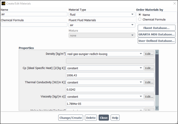
When any of the cubic equation of state models is enabled, enter the following material properties in the dialog box:
ideal specific heat
molecular weight
standard state entropy
reference temperature
critical temperature
critical pressure
critical specific volume
acentric factor
Important: Your inputs for the specific heat in the Materials dialog box will now be used to compute the ideal property functions  ,
,  , and
, and  in Equation 8–89, Equation 8–93, and Equation 8–95, respectively. In Ansys Fluent the
departure properties will be computed and added to the ideal part,
to yield the real gas specific heat, enthalpy, and entropy.
in Equation 8–89, Equation 8–93, and Equation 8–95, respectively. In Ansys Fluent the
departure properties will be computed and added to the ideal part,
to yield the real gas specific heat, enthalpy, and entropy.
Mixtures
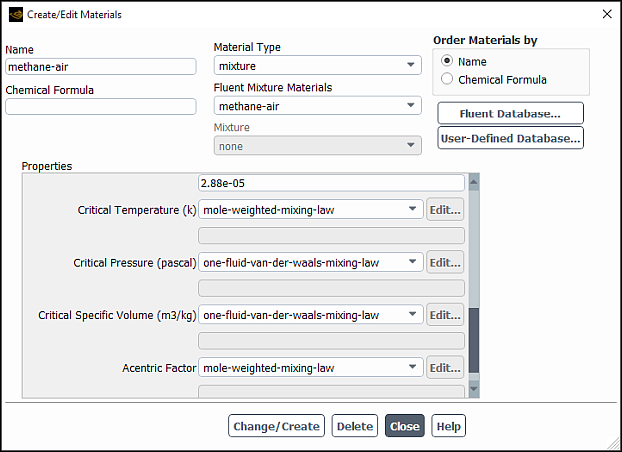
When one of the cubic equation of state models is selected from the Density drop-down list, specify the following material properties for the mixture material in the dialog box:
ideal specific heat
critical temperature
critical pressure
critical specific volume
acentric factor
You also need to enter the following material properties for each of the mixture components in the dialog box:
molecular weight
standard state entropy
reference temperature
When you are modeling a real-gas mixture, the following methods are available for the mixture critical constants:
constant: defines a constant critical temperature, critical pressure, critical specific volume, or acentric factor for the mixture material.
mole-weighted-mixing-law: applies Equation 8–97 for critical temperature, critical pressure, critical specific volume, or acentric factor for the mixture material.
one-fluid-van-der-waals-mixing-law applies Equation 8–100 and Equation 8–101 for the mixture critical temperature (depending on the real-gas model), Equation 8–102 for the mixture critical pressure, and Equation 8–103 for the mixture molar volume.
Important:
Ensure to click the button so that all the above mentioned properties are uploaded and are visible in the interface.
If you have selected mixing-law for the mixture ideal specific heat you will also need to enter the ideal specific heat values for the individual mixture components. If you have not selected constant as the option for any of the critical properties, you must enter the corresponding pure component critical properties for the mixture components.
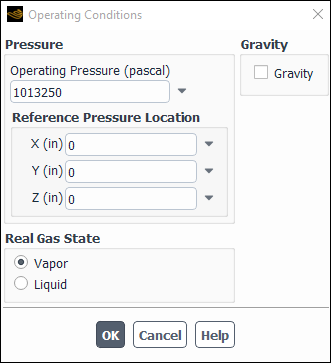
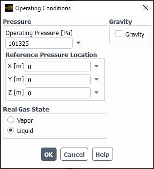
If the operating conditions in your model are in the subcritical regime, select
Vapor or Liquid as the Real Gas
State in the Operating Conditions dialog box (Figure 8.43: The Operating Conditions for a Real Gas State). Alternatively, you can use the
define/operating-conditions/set-state text command. Note that
the default is Vapor and therefore Vapor is
assumed if no changes are made to the Real Gas State settings. If
the operating conditions in your model are entirely in the supercritical regime, this
setting will have no effect.
In addition, you may specify the state for a specific fluid zone or a specific phase (if you are using multiphase modeling) by typing the following text command at the Ansys Fluent console prompt:
>define boundary-conditions modify-zones change-zone-stateSelect a name/id from fluid zones list [(liquid-zone fluid-1)]liquid-zoneSet zone real-gas state: -1:use global setting 0:liquid 1:vapor [-1]0
The flow modeling of real-gas flow is more complex and challenging than simple ideal-gas flow. Therefore, the solution might converge at a slower rate with real-gas flow than when running ideal-gas flow. It is recommended that you first attempt to converge your solution using first-order discretization then switch to second-order discretizations and re-iterate to convergence.
Special considerations apply if the operating regime in your
model is fully or partly subcritical, where the physical state may
be vapor, liquid, or a vapor/liquid mixture. In the cubic EOS real-gas
model, the phase state is determined by the selection of the cubic
root to calculate the molar-volume. This is illustrated in Figure 8.44: The PV Diagram for the Cubic Equation of State Real Gas Model, which shows a pressure versus
molar volume (PV) diagram, with a subcritical isotherm ABFED at temperature
T calculated from a cubic EOS. Curve C1CC2 represents the critical
isotherm and curve ACD the saturation dome. Points A, F, and D represent
the three roots of the EOS at the saturation pressure Ps, where A
corresponds to the molar volume of saturated liquid, D to the molar
volume of saturated vapor and point F does not have a physical significance.
Points A1 and D1 correspond to the liquid and vapor molar volumes
at pressure P1, which is lower than the saturation pressure. The liquid
and vapor molar volumes at pressure P2, which is higher than the saturation
pressure, are marked as A2 and D2 respectively. Points B and E, where
the partial derivatives of pressure with respect to volume  are
0, are called spinodal points. The loci of these points for all subcritical
temperatures, the spinodal curve, is shown with the dashed curve BCE
and sets the boundary beyond which the equation of state is no longer
valid, because the local derivative of pressure with respect to volume
becomes positive. State points inside the dome, up to the spinodal
curve, are called “metastable” because normally they
only exist temporarily in small local regions until phase change occurs.
are
0, are called spinodal points. The loci of these points for all subcritical
temperatures, the spinodal curve, is shown with the dashed curve BCE
and sets the boundary beyond which the equation of state is no longer
valid, because the local derivative of pressure with respect to volume
becomes positive. State points inside the dome, up to the spinodal
curve, are called “metastable” because normally they
only exist temporarily in small local regions until phase change occurs.
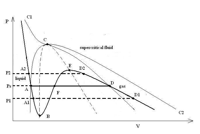
It is important to realize that the current implementation of the cubic equations of state real gas model does not determine the saturation conditions and does not model the two-phase flow where liquid and vapor coexist. In the subcritical regime and for conditions where the cubic EOS has three roots, the phase state selection is controlled by your input of Vapor or Liquid for Real Gas State in the Operating Conditions dialog box (Figure 8.43: The Operating Conditions for a Real Gas State). The default setting is Vapor, which corresponds to the state points to the right of the vapor spinodal. With reference to Figure 8.44: The PV Diagram for the Cubic Equation of State Real Gas Model, for the operating point at temperature T and pressure P1, if the Real Gas State is set to Vapor, the molar volume at point D1, which corresponds to superheated vapor, will be selected in the calculation. On the other hand, if you have selected Liquid, the molar volume of point A1 will be taken, and the corresponding state will be metastable superheated liquid. Similarly for pressure P2, which is higher than the saturation pressure Ps, if you select Liquid for Real Gas State, the liquid molar volume at A2 will be computed, and if you select Vapor the molar volume will correspond to the subcooled vapor state point D2.
In case the calculations fall inside the saturation dome, the solver will not limit the solution, but if conditions are predicted that extend beyond the vapor spinodal curve a warning will be issued:
temperature is below the spinodal point in 12 cells on zone 3.
Cubic equations of state real gas models are not available for
two-phase flows but can be applied to conditions of supercritical
pressure  and subcritical temperature
  , where the fluid is in the liquid state,
and the supercritical liquid co-exists with gas and supercritical
fluid in the same simulation. In those cases, phase change may take
place, without any of the flow conditions falling inside the saturation
dome.
, where the fluid is in the liquid state,
and the supercritical liquid co-exists with gas and supercritical
fluid in the same simulation. In those cases, phase change may take
place, without any of the flow conditions falling inside the saturation
dome.
For multicomponent simulations, when Diffusion Energy
Source is enabled in the Species Model dialog box, the species energy diffusion is by default suppressed
in the supercritical liquid regime and across the gas-liquid boundary.
The diffusion energy source can be included in the liquid regime using
the define/models/species/liquid-energy-diffusion? text command.
If your simulation contains a liquid stream, the appropriate modeling approach in the various operating condition regimes is as follows:
For
 a liquid phase does not exist.
In the region
 , you can define the flow streams directly in the boundary conditions by setting the appropriate pressure and temperature and the properties will be computed directly by the cubic EOS.
 For
 or
or  , a stream can exist in liquid phase when its temperature
  . If you would like to model phase change in this regime, the following recommendations apply:
The DPM droplet and multicomponent models are adequate and recommended for the conditions away from the critical point. This regime can be defined as
 , where the liquid physical properties can be assumed
independent of pressure.
, where the liquid physical properties can be assumed
independent of pressure.The region
 is characterized by near-critical-point
phenomena, such as strong liquid density and specific heat dependence
on both temperature and pressure. The DPM model can also be used in
this regime, but you should be cautious, as it will not take into
consideration the near-critical-point behavior. In addition, the applicability
of the evaporation and boiling rate equations is questionable in this
regime.
is characterized by near-critical-point
phenomena, such as strong liquid density and specific heat dependence
on both temperature and pressure. The DPM model can also be used in
this regime, but you should be cautious, as it will not take into
consideration the near-critical-point behavior. In addition, the applicability
of the evaporation and boiling rate equations is questionable in this
regime.If the pressure in your model is above the critical point, it is recommended to use the compressible-liquid method for Density of the droplet material.
The temperature  gives an indication of the maximum droplet temperature for applicability of the DPM models for each droplet material. These temperature limits are listed in Table 8.2: Temperature Limits for Droplet Materials in Ansys Fluent Database prodb.scm for many of the droplet materials in Ansys Fluent's
 propdb.scm materials database. For supercritical pressures ( ), the DPM models can still be used provided the droplet temperatures remain below the limit
  .
.
Table 8.2: Temperature Limits for Droplet Materials in Ansys Fluent Database prodb.scm
| Material | Tc (K) | Pc (MPa) | Normal BP (K) | Tlim (K) |
| Argon | 150.86 | 4.89 | 87.30 | 135.77 |
| Benzene | 562.00 | 4.89 | 353.00 | 505.80 |
| Helium | 5.30 | 0.23 | 4.20 | 4.77 |
| Hydrogen | 32.98 | 1.30 | 20.40 | 29.68 |
| Methyl-alcohol | 512.00 | 8.10 | 338.00 | 460.80 |
| Heptanes | 540.00 | 2.74 | 371.00 | 486.80 |
| Hexane | 507.00 | 3.02 | 342.00 | 456.30 |
| Octane | 569.00 | 2.49 | 399.00 | 512.10 |
| Pentane | 470.00 | 3.37 | 309.00 | 423.00 |
| Nitrogen | 126.00 | 3.40 | 77.40 | 113.40 |
| Oxygen | 154.00 | 5.04 | 90.20 | 138.60 |
| Toluene | 592.00 | 4.11 | 384.00 | 532.80 |
| Water | 647.00 | 22.00 | 373.00 | 582.30 |
For high pressure simulations the boiling point will be different from the normal boiling point, and for varying pressure applications the boiling point will vary with the droplet location in the domain.
When a cubic equation of state real gas model is enabled in a simulation that includes evaporating droplet particles, the boiling point is calculated from the vapor pressure data directly, as the temperature where the saturation vapor pressure equals the domain pressure. In addition, the latent heat of the evaporating or boiling droplet will vary with the droplet temperature.
The latent heat at temperature  is given by
 | (8–104) |
where  is the normal boiling point and
  is the latent heat
at the normal boiling point.
is the latent heat
at the normal boiling point.
In the Create/Edit Materials dialog box you must enter the Normal Boiling Point (NBP) and the Latent Heat at NBP for the droplet-particle Material Type. These inputs will be used for calculating the Latent Heat at the reference temperature (see Equation 12–509) and the latent heat in the droplet energy balance during vaporization and boiling according to Equation 8–104.
Important: The constant property option is disabled for the Saturation Vapor Pressure property when a real gas model is used in the simulation. Also, ensure to enter the appropriate droplet saturation vapor pressure data to cover the complete pressure/temperature range in your model.
Finally when a cubic equation of state real-gas model is enabled in a simulation with droplet models, the condition for switching from the vaporization to the boiling law will be
 | (8–105) |
where  is the saturation vapor pressure and P is the domain pressure. If
  while in the boiling law, the model will switch back to the vaporization law. Under supercritical pressure conditions (
 ), the vaporization models are applicable at droplet temperatures below the critical point, and the switching condition from vaporization to boiling
  is never met because the vapor pressure curve is defined only up to the critical point.
For the multicomponent droplets in the supercritical pressure regime, failure of the saturation temperature calculation algorithm may indicate that the droplet has approached the critical temperature, provided that you have entered accurate vapor pressure data for all components. In such a case, you can use the following text command:
define/models/dpm/options/treat-multicomponent-saturation-temperature-failure?
Dump multicomponent particle mass if the saturation temperature
              calculation fails? [no]
y
When this option is enabled, Ansys Fluent dumps the particle mass into the continuous phase if the saturation temperature calculation fails.
All postprocessing functions properly report and display the current thermodynamic and transport properties of the selected real gas model. The thermodynamic and transport properties controlled by the cubic equations of state real gas model include the following:
density
enthalpy
entropy
sound speed
specific heat
any quantities that are derived from the properties listed above (for example, total quantities, ratio of specific heats)
In addition to the properties listed above, you can also report
compressibility factor
reduced temperature
reduced pressure
spinodal temperature
subcritical condition
If you are modeling a real-gas mixture you can report the composition-dependent mixture critical properties
critical temperature
critical pressure
critical specific volume
acentric factor
The NIST real gas models use the National Institute of Standards and Technology (NIST) Thermodynamic and Transport Properties of Refrigerants and Refrigerant Mixtures Database Version 10.0 (REFPROP v10.0) to evaluate thermodynamic and transport properties of approximately 152 fluids or a mixture of these fluids.
The REFPROP v10.0 database is a shared library that is dynamically loaded into the solver when you enable one of the NIST real gas models in an Ansys Fluent session. Once the NIST real gas model is activated, control of relevant property evaluations is relinquished to the REFPROP database. All postprocessing functions will properly report and display the current thermodynamic and transport properties of the real gas.
The following limitations exist for the NIST real gas model:
The NIST real gas model assumes that the fluid you will be using in your Ansys Fluent computation is superheated vapor, supercritical fluid, or liquid. Note that subcritical flow conditions, where vapor coexists with liquid in two-phase flow, are not supported. In addition, all fluid zones must contain the real gas; you cannot include a real gas and another fluid in the same problem.
Pressure-inlet, mass flow-inlet, and pressure-outlet are the only inflow and outflow boundaries available for use with the real gas models.
Non-reflecting boundary conditions are not compatible with the real gas models when using the density-based solver. If your model requires NRBC and a real gas model, you must use the pressure-based solver.
The mixture flow does not permit chemical reactions with the NIST real gas model.
The multicomponent NIST real gas models cannot be used with any of the multiphase models. You can, however, use a NIST material in single-component multiphase flows. The model is compatible with the Lagrangian Dispersed Phase Models only for the massless and inert particle types.
You cannot modify material properties in the REFPROP database libraries, or add custom materials to the NIST real gas model.
Only one pure fluid or one multiple-species mixture in a simulation may use the NIST real gas model. Multiple NIST materials may be created, but those participating in the simulation must all refer to a unique NIST fluid. This is a third-party limitation of the NIST/REFPROP module.
The NIST real gas model supports 152 fluids from the REFPROP database. These include pure
fluids (with the file extension .FLD) and pseudo-fluids (with the
file extension .PPF). The fluids that are supported by REFPROP
v10.0 and used in the NIST real gas model are listed in Table 8.3: v10.0 (the corresponding property file name appears in
parentheses, where it does not coincide with the fluid name).
The REFPROP v10.0 database employs accurate pure-fluid equations of state that are available from NIST. These equations are based on three models:
modified Benedict-Webb-Rubin (MBWR) equation of state
Helmholtz-energy equation of state
extended corresponding states (ECS)
For a fluid that consists of a multispecies-mixture the thermodynamic properties are computed by employing mixing-rules applied to the Helmholtz energy of the mixture components.
Important: The database does not include transport property models for the species marked with * in Table 8.3: v10.0. As a result the NIST real gas model with those species can only be used for modeling inviscid flow.
Table 8.3: v10.0
| Short Name | Full Name | Fluid Data File |
|---|---|---|
| Butene | 1-Butene | 1BUTENE.FLD |
| 1-Butyne | But-1-yne | 1BUTYNE.FLD |
| 1-Pentene | Pent-1-en | 1PENTENE.FLD |
| 3-Methylpentane | 3-Methylpentane | 3METHYLPENTANE.FLD |
| 1,3-Butadiene | Buta-1,3-diene | 13BUTADIENE.FLD |
| 2,2-Dimethylbutan | 2,2-Dimethylbutan | 22DIMETHYLBUTANE.FLD |
| 2,3-Dimethylbutan | 2,3-Dimethylbutan | 23DIMETHYLBUTANE.FLD |
| Acetone | Propanone | ACETONE.FLD |
| Acetylene | Ethyne | ACETYLENE.FLD |
| Ammonia | Ammonia | AMMONIA.FLD |
| Argon | Argon | ARGON.FLD |
| Benzene | Benzene | BENZENE.FLD |
| Butane | n-Butane | BUTANE.FLD |
| Methylcyclohexane | Methylcyclohexane | C1CC6.FLD |
| cis-Butene | cis-2-Butene | C2BUTENE.FLD |
| Propylcyclohexane | n-Propylcyclohexane | C3CC6.FLD |
| Perfluorobutane | Decafluorobutane | C4F10.FLD |
| Perfluoropentane | Dodecafluoropentane | C5F12.FLD |
| Perfluorohexane | Tetradecafluorohexane | C6F14.FLD |
| Undecane | Undecane | C11.FLD |
| Dodecane | Dodecane | C12.FLD |
| Hexadecane | Hexadecane | C16.FLD |
| Docosane | Docosane | C22.FLD |
| R13I1 | Trifluoroiodomethane | CF3I.FLD |
| Chlorine | Chlorine | CHLORINE.FLD |
| Chlorobenzene | Chlorobenzene | CHLOROBENZENE.FLD |
| Carbon monoxide | Carbon monoxide | CO.FLD |
| Carbon dioxide | Carbon dioxide | CO2.FLD |
| Carbonyl sulfide | Carbon oxide sulfide | COS.FLD |
| Cyclobutene | 1-Cyclobutene | CYCLOBUTENE.FLD |
| Cyclohexane | Cyclohexane | CYCLOHEX.FLD |
| Cyclopentane | Cyclopentane | CYCLOPEN.FLD |
| Cyclopropane | Cyclopropane | CYCLOPRO.FLD |
| Deuterium | Deuterium | D2.FLD |
| Heavy water | Deuterium oxide | D2O.FLD |
| D4 | Octamethylcyclotetrasiloxane | D4.FLD |
| D5 | Decamethylcyclopentasiloxane | D5.FLD |
| D6 | Dodecamethylcyclohexasiloxane | D6.FLD |
| Diethanolamine | 2,2'-Iminodiethanol | DEA.FLD |
| Decane | Decane | DECANE.FLD |
| Diethyl ether | Diethyl ether | DEE.FLD |
| Dimethyl carbonate | Dimethyl ester carbonic acid | DMC.FLD |
| Dimethyl ether | Methoxymethane | DME.FLD |
| Ethylbenzene | Phenylethane | EBENZENE.FLD |
| Ethylene glycol | 1,2-Ethandiol | EGLYCOL.FLD |
| Ethane | Ethane | ETHANE.FLD |
| Ethanol | Ethyl alcohol | ETHANOL.FLD |
| Ethylene | Ethene | ETHYLENE.FLD |
| Ethylene oxide | Ethylene oxide | ETHYLENEOXIDE.FLD |
| Ethylene oxide | Fluorine | FLUORINE.FLD |
| Hydrogen sulfide | Hydrogen sulfide | H2S.FLD |
| Hydrogen chloride | Hydrogen chloride | HCL.FLD |
| Helium | Helium-4 | HELIUM.FLD |
| Heptane | Heptane | HEPTANE.FLD |
| Hexane | Hexane | HEXANE.FLD |
| Hydrogen (normal) | Hydrogen (normal) | HYDROGEN.FLD |
| Isobutene | 2-Methyl-1-propene | IBUTENE.FLD |
| Isohexane | 2-Methylpentane | IHEXANE.FLD |
| Isooctane | 2,2,4-Trimethylpentane | IOCTANE.FLD |
| Isopentane | 2-Methylbutane | IPENTANE.FLD |
| Isobutane | 2-Methylpropane | ISOBUTAN.FLD |
| Krypton | Krypton | KRYPTON.FLD |
| MD2M | Decamethyltetrasiloxane | MD2M.FLD |
| MD3M | Dodecamethylpentasiloxane | MD3M.FLD |
| MD4M | Tetradecamethylhexasiloxane | MD4M.FLD |
| MDM | Octamethyltrisiloxane | MDM.FLD |
| Monoethanolamine | Ethanolamine | MEA.FLD |
| Methane | Methane | METHANE.FLD |
| Methanol | Methanol | METHANOL.FLD |
| Methyl linoleate | Methyl (Z,Z)-9,12-octadecadienoate | MLINOLEA.FLD |
| Methyl linolenate | Methyl (Z,Z,Z)-9,12,15-octadecatrienoate | MLINOLEN.FLD |
| MM | Hexamethyldisiloxane | MM.FLD |
| Methyl oleate | Methyl cis-9-octadecenoate | MOLEATE.FLD |
| Methyl palmitate | Methyl hexadecanoate | MPALMITA.FLD |
| Methyl stearate | Methyl octadecanoate | MSTEARAT.FLD |
| m-Xylene | 1,3-Dimethylbenzene | MXYLENE.FLD |
| Nitrous oxide | Dinitrogen monoxide | N2O.FLD |
| Neon | Neon | NEON.FLD |
| Neopentane | 2,2-Dimethylpropane | NEOPENTN.FLD |
| Nitrogen trifluoride | Nitrogen trifluoride | NF3.FLD * |
| Nitrogen | Nitrogen | NITROGEN.FLD |
| Nonane | Nonane | NONANE.FLD |
| Novec 649, 1230 |
1,1,1,2,2,4,5,5,5-Nonafluoro-4-(trifluoromethyl)-3- pentanone | NOVEC649.FLD |
| Octane | Octane | OCTANE.FLD |
| Orthohydrogen | Orthohydrogen | ORTHOHYD.FLD * |
| Oxygen | Oxygen | OXYGEN.FLD |
| o-Xylene | 1,2-Dimethylbenzene | OXYLENE.FLD |
| Parahydrogen | Parahydrogen | PARAHYD.FLD |
| Pentane | Pentane | PENTANE.FLD |
| Propadiene | 1,2-Propadiene | PROPADIENE.FLD |
| Propane | Propane | PROPANE.FLD |
| Propylene | Propene | PROPYLEN.FLD |
| Propylene oxide | 1,2-Epoxypropane | PROPYLENEOXIDE.FLD |
| Propyne | Propyne | PROPYNE.FLD |
| p-Xylene | 1,4-Dimethylbenzene | PXYLENE.FLD |
| R11 | Trichlorofluoromethane | R11.FLD |
| R12 | Dichlorodifluoromethane | R12.FLD |
| R13 | Chlorotrifluoromethane | R13.FLD |
| R14 | Tetrafluoromethane | R14.FLD |
| R21 | Dichlorofluoromethane | R21.FLD |
| R22 | Chlorodifluoromethane | R22.FLD |
| R23 | Trifluoromethane | R23.FLD |
| R32 | Difluoromethane | R32.FLD |
| R40 | Methyl chloride | R40.FLD |
| R41 | Fluoromethane | R41.FLD |
| R113 | 1,1,2-Trichloro-1,2,2-trifluoroethane | R113.FLD |
| R114 | 1,2-Dichloro-1,1,2,2-tetrafluoroethane | R114.FLD |
| R115 | Chloropentafluoroethane | R115.FLD |
| R116 | Hexafluoroethane | R116.FLD |
| R123 | 2,2-Dichloro-1,1,1-trifluoroethane | R123.FLD |
| R124 | 1-Chloro-1,2,2,2-tetrafluoroethane | R124.FLD |
| R125 | Pentafluoroethane | R125.FLD |
| R134a | 1,1,1,2-Tetrafluoroethane | R134A.FLD |
| R141b | 1,1-Dichloro-1-fluoroethane | R141B.FLD |
| R142b | 1-Chloro-1,1-difluoroethane | R142B.FLD |
| R143a | 1,1,1-Trifluoroethane | R143A.FLD |
| Dichloroethane | 1,2-Dichloroethane | R150.FLD |
| R152a | 1,1-Difluoroethane | R152A.FLD |
| R161 | Fluoroethane | R161.FLD |
| R218 | Octafluoropropane | R218.FLD |
| R227ea | 1,1,1,2,3,3,3-Heptafluoropropane | R227EA.FLD |
| R236ea | 1,1,1,2,3,3-Hexafluoropropane | R236EA.FLD |
| R236fa | 1,1,1,3,3,3-Hexafluoropropane | R236FA.FLD |
| R245ca | 1,1,2,2,3-Pentafluoropropane | R245CA.FLD |
| R245fa | 1,1,1,3,3-Pentafluoropropane | R245FA.FLD |
| R365mfc | 1,1,1,3,3-Pentafluorobutane | R365MFC.FLD |
| R1123 | Trifluoroethylene | R1123.FLD |
| R1216 | Hexafluoropropene | R1216.FLD |
| R1224yd(Z) | (Z)-1-Chloro-2,3,3,3-tetrafluoropropene | R1224YDZ.FLD |
| R1233zd(E) | trans-1-Chloro-3,3,3-trifluoro-1-propene | R1233ZDE.FLD |
| R1234yf | 2,3,3,3-Tetrafluoroprop-1-ene | R1234YF.FLD |
| R1234ze(E | trans-1,3,3,3-Tetrafluoropropene | R1234ZEE.FLD |
| R1234ze(Z) | cis-1,3,3,3-Tetrafluoropropene | R1234ZEZ.FLD |
| R1243zf | 3,3,3-Trifluoropropene | R1243ZF.FLD |
| R1336mzz(Z) | (Z)-1,1,1,4,4,4-Hexafluoro-2-butene | R1336MZZZ.FLD |
| RC318 | Octafluorocyclobutane | RC318.FLD |
| RE143a | Methyl trifluoromethyl ether | RE143A.FLD |
| RE245cb2 | Methyl-pentafluoroethyl-ether | RE245CB2.FLD |
| RE245fa2 | 2,2,2-Trifluoroethyl-difluoromethyl-ether | RE245FA2.FLD |
| RE347mcc (HFE-7000) | 1,1,1,2,2,3,3-Heptafluoro-3-methoxypropane | RE347MCC.FLD |
| Sulfur hexafluoride | Sulfur hexafluoride | SF6.FLD |
| Sulfur dioxide | Sulfur dioxide | SO2.FLD |
| trans-Butene | trans-2-Butene | T2BUTENE.FLD |
| Toluene | Methylbenzene | TOLUENE.FLD |
| Vinyl chloride | Chloroethylene | VINYLCHLORIDE.FLD |
| Water | Water | WATER.FLD |
| Xenon | Xenon | XENON.FLD |
| Air (dry) | Nitrogen + oxygen + argon (0.7812/0.2096/0.0092) | AIR.PPF |
| R404A | 44% R125/4% R134a/52% R143a | R404A.PPF * |
| R407C | 23% R32/25% R125/52% R134a | R407C.PPF * |
| R410A | 50% R32/50% R125 | R410A.PPF * |
| R507A | 50% R125/50% R143a | R507A.PPF * |
The NIST real gas model can be enabled for pure fluids by selecting
real-gas-nist for Density on the
Create/Edit Materials dialog box.
![]() Physics →
Materials → Create/Edit...
Physics →
Materials → Create/Edit...
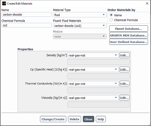
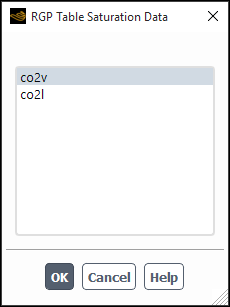
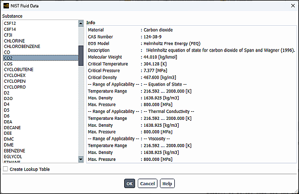
When you select Edit… for Density, you will be prompted to select the appropriate NIST data from the NIST Fluid Data dialog box. After selecting a valid fluid, properties for the specified material, including its applicable pressure and temperature ranges, will be displayed.
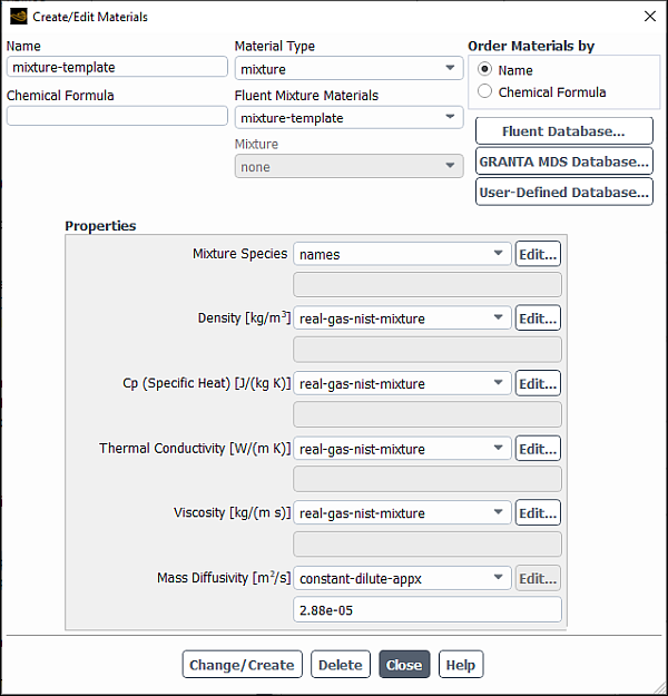
For multiple-species mixtures, enable the Species Transport model and specify the number and names of species, as described in Enabling Species Transport and Reactions and Choosing the Mixture Material. Then on the Create/Edit Materials dialog box, select real-gas-nist-mixture for Density.
Afterwards, you must select the appropriate NIST fluid data for each species as you would for a pure fluid.
Important:
For mixture flows, not all combinations of species mixtures are allowed. This could be due to lack of data for one or more binary pairs. In such situations an error message generated by NIST will be returned and displayed on the Ansys Fluent console, and no real gas material is allowed to be created. In some combinations the mixing data will be estimated, a warning message will be displayed on the Ansys Fluent console and the mixture material allowed to be created.
Transport property calculations are not supported for mixtures that include water with molar concentration over 5%. If this limit is exceeded in your calculation, Ansys Fluent will issue a warning message. Transport equations are not available for the ammonia/water mixture and for mixtures with alcohols. As a result, the NIST real gas model with those mixtures can only be used for modeling inviscid flow.
Cp (Specific Heat), Thermal Conductivity, and Viscosity will be automatically set respectively to real-gas-nist (pure fluid) or real-gas-nist-mixture (multiple species mixture).
If you want to use NIST lookup tables in your simulation, you can create them as described in Creating NIST Look-up Tables.
If your case contains no NIST tables, and you would like to model flow in the liquid state, you can set the Real Gas State to liquid in the Operating Conditions dialog box.
In addition, you may specify the state for specific fluid zones or a specific phase (if you are using the multiphase model) by typing the following text command in the Ansys Fluent console prompt:
>define boundary-conditions modify-zones change-zone-stateSelect a name/id from fluid zones list [(liquid-zone fluid-1)]liquid-zoneSet zone real-gas state: -1:use global setting 0:liquid 1:vapor [-1]0
By default, the NIST functions are called directly each time the thermal properties are updated during an iteration. Alternatively, you can use NIST look-up tables in your simulation as described below. Computing the look-up table reduces the computation time because the NIST functions do not need to be called each time the thermal properties are updated.
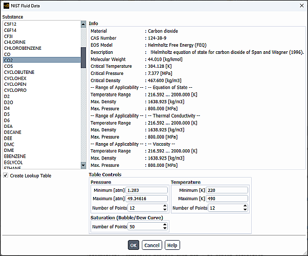
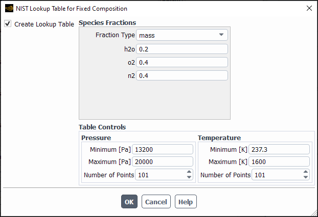
To create a full NIST look-up table, first enable the NIST real gas model as described in Using the NIST Real Gas Models, and then select Create Lookup Table.
For both single and multi-species real gas models, you need to specify:
Pressure and Temperature bounds for the table.
You must ensure that the temperature and pressure bounds you specify are strictly within the stated limits of applicability that are displayed when selecting the NIST fluid data.
Number of pressure and temperature points.
The minimum number of pressure and temperature points is 12 and there is no upper limit. However, the larger the table, the greater the memory and computing time requirements. It is advised to perform test runs to balance the costs (memory and computing time) and accuracy.
For single-species, you also need to specify the number of points for Saturation (Bubble/Dew Curve) properties.
For multi-species, you also need to specify the mixture composition on a mass or mole basis. You must ensure that the sum of all constituent fractions add up to 1 when specifying mass/molar fractions for the components. The maximum number of species is 20.
If properties are needed at conditions outside the limits you have specified for the table, Fluent automatically calls the original NIST model functions to calculate the thermal properties. If more than 10% of the property evaluations require computation outside the look-up table, Fluent prints a message indicating the percentage of calculations using direct computation. This can be used as an indicator to adjust the temperature and pressure ranges for the table to minimize the computational cost.
For computation of saturation properties for the bubble and dew points for a single- or multiple-species, Fluent provides macros that you can use in UDFs. See NIST Real Gas Saturation Properties for more information.
Look-up tables apply for compressible fluids with material properties that are a function of local pressure and temperature. The material properties covered by the table include fluids in the liquid and vapor phases. Flashing applications between liquid and vapor phases can be conducted using saturation conditions established for the fluid(s) using mass transfer models.
Look-up tables and saturation tables are created for fixed fluid compositions. This means the look-up tables are based on the following assumptions:
Mixture composition is constant.
No chemical reactions are involved.
No mixing of fluids of different compositions, including no mixing between phases.
Look-up tables only apply to single-species/multi-species in single-phase flows
The temperature and pressure bounds must be specified within the stated limits of applicability that are displayed when the NIST model is loaded.
When specifying the look-up table size, it is important to pick temperature and pressure ranges that are large enough to satisfy the current flow conditions.
If the temperature and pressure ranges you specify are too narrow, Fluent uses the NIST model to calculate thermal properties. The time saved by creating the table will be negated if the percentage of calculations performed outside of the table is greater than 10%. This percentage is printed, so you can use it as an indicator for adjusting the temperature and pressure range of the table.
The look-up table is a structured table and may not be suitable for simulating flow behaviors near the critical point when higher resolution is required.
When you enable one of the NIST real gas models (pure fluid or multiple-species mixture) using the legacy TUI and select a valid material, Ansys Fluent’s functionality remains the same as when you model fluid flow and heat transfer using an ideal gas, with the exception of the Create/Edit Materials Dialog Box.
When you enable one of the NIST real gas models (pure fluid or multiple-species mixture) through the legacy TUI, the following limitations apply in addition to those listed in Limitations of the NIST Real Gas Models:
When you are using the NIST real gas models, the NIST materials defined in your simulation will appear in the Create/Edit Materials Dialog Box either with the name real-gas-
_name, where_nameis the NIST material selected for the single species model, or with the name real-gas-mixture for the multiple species model. The inputs for the properties calculated by the NIST functions are disabled. You can use the Create/Edit Materials Dialog Box to define or modify:Mass diffusivity property in the real-gas-mixture material if you are using the multiple-species NIST real gas model (note that the kinetic-theory option is not available)
Radiation properties if you are modeling radiation
Properties of materials other than the NIST real-gas-mixture or real-gas-fluid materials
Activating one of the NIST real gas models is a two-step process. First you enable either the single- or multi-species NIST real gas model, and then you select the fluid material from the REFPROP database.
Enable the appropriate NIST real gas model by typing the following text command at the Ansys Fluent console prompt:
Pure fluid real gas model:
>
define/user-defined/real-gas-models/nist-real-gas-modeluse NIST real gas? [no]yesMulti-species real gas model:
>
define/user-defined/real-gas-models/nist-multispecies-real-gas-modeluse multispecies NIST real gas? [no]yes
The list of available pure fluid materials you can select from will be displayed.
Select material from the REFPROP database list:
Pure fluid real gas model:
Enter the name of a single pure fluid that you want to investigate as follows:
select real-gas data file [""]
methane.fldMulti-species real gas model:
Enter the number of desired species in the mixture:
Number of species []
3followed by the name of each fluid in quotation marks selected from the list printed in the console:
select real-gas data file [""]
nitrogen.fldselect real-gas data file [""]co2.fldselect real-gas data file [""]methane.fldUpon selection of a valid pure or multi-species fluids, Ansys Fluent will load the relevant material data from a library of pure fluids supported by the REFPROP database, and report that it is opening the shared library (
librealgas.so) where the compiled REFPROP database source code is located. A list of properties for the specified material, including its applicable pressure and temperature ranges, will also be reported in the console.
Important:For mixture flows, not all combinations of species mixtures are allowed. This could be due to lack of data for one or more binary pairs. In such situations an error message generated by NIST will be returned and displayed on the Ansys Fluent console, and no real gas material is allowed to be created. In some combinations the mixing data will be estimated, a warning message will be displayed on the Ansys Fluent console and the mixture material allowed to be created.
Transport property calculations are not supported for mixtures that include water with molar concentration over 5%. If this limit is exceeded in your calculation, Ansys Fluent will issue a warning message. Transport equations are not available for the ammonia/water mixture and for mixtures with alcohols. As a result, the NIST real gas model with those mixtures can only be used for modeling inviscid flow.
If you want to use NIST lookup tables in your simulation, you can create them as described in the following sections:
Creating Full NIST Look-up Tables (single and multi-species materials with thermal properties as well as saturation data for a fixed multi-species composition)
Creating Binary Mixture Saturation Tables for Binary Mixtures (binary mixtures only)
(cases with no NIST tables only) If you would like to model flow in the liquid state, you can use the
set-stateTUI command. Note that the default state is vapor, so if you do not go through this step, vapor is assumed. Also, if the flow conditions do not permit liquid to exist, a vapor calculation will be performed instead.>
define/user-defined/real-gas-models/set-stateSelect vapor state (else liquid)?[yes]In addition, you may specify the state for a specific fluid zone or a specific phase (if you are using the multiphase model) by typing the following text command at the Ansys Fluent console prompt:
>
define boundary-conditions modify-zones change-zone-stateSelect a name/id from fluid zones list [(liquid-zone fluid-1)]liquid-zoneSet zone real-gas state: -1:use global setting 0:liquid 1:vapor [-1]0
By default, the NIST functions are called directly each time the thermal properties are updated during iteration. Alternatively, you can use the NIST look-up tables in your simulation as described below. Computing the look-up table offers two advantages:
Reduction in computation time because the NIST functions do not need to be called each time the thermal properties are updated
The look-up table created is applicable to both liquid and vapor phases
To create a full NIST look-up table, first enable the NIST real gas model as described in Activating the NIST Real Gas Model, and then follow these steps:
When prompted with
Create Full NIST LookUp Tables for multi components? [no], answeryes.Specify parameters for the look-up table generation.
For both single- and multi-species real gas models, you need to specify:
Pressure and temperature bounds for the table
You must ensure that the temperature and pressure bounds you specify are strictly within the stated limits of applicability that are displayed when the NIST model is loaded.
Number of pressure, temperature, and saturation points, which determines the resolution of the property look-up table
The minimum number of pressure and temperature points is 12 and there is no upper limit. However, the larger the table, the greater the memory and computing time requirements. Use a few test runs to strike the best balance of costs (memory and computing time) and accuracy.
For multi-species, you will also need to specify:
Upper and lower molar density bounds for bubble and dew point calculations
Molar density is used to build the saturation table. The default values work well for most compositions.
The mixture composition on a mass or mole basis
You must ensure that the sum of all constituent fractions adds up to 1 when specifying mass/molar fractions for the components. The maximum number of species is 20.
The bubble points and dew points filenames and the directory where you want to store the files.
Examples of inputs for the NIST look-up tables:
Pure fluid real gas model:
Min Pressure Value For NIST Table (pa) [13200] Max Pressure Value For NIST Table (pa) [20000]
1000000Min Temperature Value For NIST Table (k) [237.3] Max Temperature Value For NIST Table (k) [500]400Number of Pressure Points For NIST Table [101] Number of Temperature Points For NIST Table [101] Number of Saturation Points For Bubble/Dew Curve [300] NIST table created! Properties for both liquid and vapor phases included! Tcrit = 3.391730e+02 pcrit = 3.617700e+06 Dcrit = 5.735823e+02 Ttrp = 1.725200e+02Multi-species real gas model:
Min Pressure Value For NIST Table (pa) [130000]
Max Pressure Value For NIST Table (pa) [5000000]
Min Temperature Value For NIST Table (k) [220] 180
Max Temperature Value For NIST Table (k) [490] 600
Number of Pressure Points For NIST Table [101]
Number of Temperature Points For NIST Table [101]
Please Select Mass Fractions [Y] or Molar Fractions [N] for Composition of Fluid
 [yes]
Composition of Fluid will be set in Mass Fractions!
co2.fld [0.4]
methane.fld [0.4] 0.6
Create NIST Saturation Curves for the same multi components?
[no] y
Number of Saturation Points For Bubble/Dew Curve [300] 22
Min Molar Density For Bubble and Dew Points Calculations (mol/l) [0.1]
Max Molar Density For Bubble and Dew Points Calculations (mol/l) [25]
Bubble Points File Name ["Bubble_PT.xy"]
Dew Points File Name ["Dew_PT.xy"]
Directory to store Saturation Files [""]
Start NIST Look-Up Table Calculations ...

Property Table... 83.3 percent completed!

NIST table for 2-components created! Properties for both liquid and vapor phases included!
End NIST Look-Up Table Calculations
Use the created NIST Lookup Table for thermal property calculations? [no] y
Once the table is created, you must confirm that you want to use the look-up table for thermal properties calculations when prompted.
Use the created NIST Lookup Table for thermal property calculations? [no]
yesThe created NIST Lookup Table will be used to calculate the thermal properties!If properties are needed at conditions outside the limits you have specified for the table, Fluent will automatically call the original NIST model functions to calculate the thermal properties. If more than 10% of the property evaluations require computation outside the look-up table, Fluent will print a message indicating the percentage of calculations using direct computation. This can be used as an indicator to adjust the temperature and pressure ranges for the table to minimize the computational cost.
For multi-species real gas properties, the following tables will be created:
fluid properties
saturation conditions
Capabilities and Limitations on Using Multi-Species Full NIST look-up Tables
The look-up table is not saved with the case file. If you restart Fluent or re-read case and data files into the current Fluent session, the table will be cleared and you must go through the steps above to re-create it before running a simulation.
For computation of saturation properties for the bubble and dew points for a single- or multiple-species, Fluent provides macros that you can use in UDFs. See NIST Real Gas Saturation Properties in the Fluent Customization Manual for more information.
The tables apply for compressible fluids with material properties that are a function of local pressure and temperature. The material properties covered by the table include fluids in the liquid and vapor phases. The flashing applications between liquid and vapor phases can be conducted using saturation conditions established for the fluid(s) using mass transfer models.
The property look-up tables and saturation tables are created for fixed fluid compositions. This means the look-up tables are based on the following assumptions:
Mixture composition is constant
No chemical reactions are involved
No mixing of fluids of different compositions, including no mixing between phases
The look-up table only applies to single-species/multi-species in single-phase flows.
The temperature and pressure bounds must be specified within the stated limits of applicability that are displayed when the NIST model is loaded.
When specifying the table size, it is important to pick temperature and pressure ranges that are large enough to satisfy the current flow conditions.
If the temperature and pressure ranges you specify are too narrow, Fluent uses the NIST model to calculate the thermal properties. The time saved by creating the table will be negated if the percentage of calculations performed outside of the table is greater than 10%. This percentage is printed, so you can use it as an indicator for adjusting the temperature and pressure range of the table.
For multi-species table, the bubble and dew points are saved into files(Fluent plot file format) called
Bubble_PT.xyandDew_PT.xyin the working directory.The look-up table is a structured table and may not be suitable for simulating flow behaviors near the critical point when higher resolution is required.
To create a saturation data look-up table for binary species mixtures (mixtures of two species only), first enable the NIST real gas model as described in Activating the NIST Real Gas Model and then follow these steps:
When prompted with
Create Full NIST LookUp Tables for multi components? [no], answerno.When prompted with
Create Saturation Table For Binary Mixture Only? [no], answeryes.Important: Not all binary mixtures can be computed from the Fluent built-in NIST model. The allowed combination of materials is determined by the current database of NIST that can be found in hmx.bnc in the Ansys Fluent installation directory.
Specify parameters for the binary saturation data look-up table generation:
The number of saturation curves
The number of points for each saturation curve
The default number is 12. The actual number of points for each bubble and dew curve may be different than specified because the NIST model may not yield valid computation results for every density point for a given mass fraction.
Upper and lower molar density bounds for bubble and dew point calculations
The molar density is used to build the saturation table. You should provide reasonable values for the minimum and maximum molar densities corresponding to gas phase at low pressure and high temperature, and liquid phase at high pressure and low temperature. The default values (as shown in the example below) are a good starting point. You may need to adjust these values if there is not enough data in the selected range.
The filenames for bubble points and dew points and the existing directory where you want to store the files.
An example of inputs for the NIST binary look-up table:
Number of Mass Fraction Points For Binary Mixture [12]
Number of Saturation Points For Bubble/Dew Curve [12]
Min Molar Density For Bubble and Dew Points Calculations (mol/l) [0.1]
Max Molar Density For Bubble and Dew Points Calculations (mol/l) [25]
Bubble Points File Name ["Bubble_PT.xy"]
Dew Points File Name ["Dew_PT.xy"]
Directory to store Saturation Files [""] out
The lookup table builds multiple sets of the bubble and dew points for the binary mixture with mass fractions for the first component between 0 and 1. The second component mass fraction is equal to the first component mass fraction subtracted from unity. The number of saturation curves is determined by the number of mass fraction points that you specified.
Once the lookup table is created, Fluent saves the bubble and dew points data into files and directory you specified.
NIST Binary Saturation Files
NIST binary saturation files store saturation data lookup table for bubble and dew points for a binary mixture with mass fractions between 0 and 1. They can be used for mass and heat transfer modeling involving phase changes.
The binary saturation file structure is as follows. The file contains several data sets for bubble/dew point curves for a series of mass fractions. Each data set consists of the following three parts:
Line 1: The mass fraction of the first species (a single float number between 0 and 1).
Line 2: The number of data pairs for saturation pressure and temperature.
The specified number of lines that follow line 2: Data pairs of saturation pressure and temperature. The last pressure-temperature pair corresponds to the critical condition.
The example below shows the saturation dew point data for the first two curves, both with 12 pressure-temperature pairs. The first data set is for 0 and the second is for a 0.083333 mass fraction of the first species. The pressure-temperature critical condition is (4.872200e+06, 3.053220e+02) for the first curve and (5.547305e+06, 2.947561e+02) for the second curve.
 0.000000
12
1.142108e+00 9.036800e+01
7.314020e+01 1.099093e+02
1.202771e+03 1.294505e+02
8.833626e+03 1.489918e+02
3.890130e+04 1.685331e+02
1.219542e+05 1.880744e+02
3.025174e+05 2.076156e+02
6.354397e+05 2.271569e+02
1.182515e+06 2.466982e+02
2.011733e+06 2.662395e+02
3.201942e+06 2.857807e+02
4.872200e+06 3.053220e+02

 0.083333
12
1.509489e+05 1.891238e+02
1.257388e+06 2.428513e+02
2.252097e+06 2.631615e+02
3.090473e+06 2.752623e+02
3.775539e+06 2.831498e+02
4.318958e+06 2.883822e+02
4.735586e+06 2.917723e+02
5.042345e+06 2.938262e+02
5.258091e+06 2.949048e+02
5.402834e+06 2.952901e+02
5.495209e+06 2.951982e+02
5.547305e+06 2.947561e+02

.....
.....
The flow modeling of NIST real-gas flow is much more complex and challenging than simple ideal-gas flow. Therefore, you should expect the solution to converge at much slower rate with real-gas flow than when running ideal-gas flow. Also due to the complexity of the equations used in property evaluations, converging a solution with the real-gas model is in general done at much lower Courant values when you are using the density-based solver, or at much lower under-relaxation values if you are using the pressure-based solver. It is recommended that you first attempt to converge your solution using first-order discretization, then switch to second-order discretizations and re-iterate to convergence.
The real-gas properties in NIST are defined within a limited/bounded range. It is important that the flow conditions you are prescribing fall within the range of the database. It is possible that you specify flow at a state that is physically valid but otherwise not defined in the database. In this situation the solution will diverge or immediately generate an error message on the Ansys Fluent console as soon as the state crosses the limit of the database. In some instances, the actual converged state is just within the bounded defined database but only transitory outside the range. In this situation the divergence can be avoided by lowering the Courant value or under-relaxation factors so a less aggressive convergence rate is adapted.
Finally, if you attempt to initialize the flow from an inlet flow conditions and an error message is generated from one of the property routines, then this is an indicator that the flow conditions you have specified is not defined within the range of the database.
When you save your completed real gas model to a case file, the linkage to the shared library
containing real gas properties will be saved to the case file (along with property data
for the material you selected in the NIST real gas model). This information can be
reported to the console by listing the material properties (using the command
/define/materials/list-properties <material-name>) and
viewed in the Create/Edit Materials dialog box by selecting
Edit… for density.
All postprocessing functions properly report and display the current thermodynamic and transport properties of the selected real gas model. The thermodynamic and transport properties controlled by the NIST real gas model include the following:
density
enthalpy
entropy
molecular weight
molecular viscosity
sound speed
specific heat
thermal conductivity In addition to the properties listed above, you can also report
compressibility factor
any quantities that are derived from the properties listed above (for example, total quantities, ratio of specific heats)
The user-defined real gas model (UDRGM) has been developed to allow you to write your own custom real gas model to fit your particular modeling needs. It also allows you to simulate a single-species flow, multiple-species mixture flow, multiphase flow, or volumetric reactions.
The following limitations exist for the UDRGM:
You cannot include more than one user-defined real gas material (fluid or mixture) in the same problem. However, you can use other materials together with real gas in your simulation.
When you are using the UDRGM, the materials defined in your real gas UDF will appear in the Create/Edit Materials Dialog Box with the name real-gas-fluid or real-gas-mixture and all physical and thermodynamic property inputs disabled. Use the Create/Edit Materials Dialog Box to define or modify:
Mass diffusivity property in the real-gas-mixture material if you are modeling multicomponent flow.
Chemical reactions in the real-gas-mixture if you are modeling reacting flow.
Radiation properties for the real-gas-mixture or the real-gas-fluid materials if you are modeling radiation.
Properties of materials other than the user-defined real-gas-mixture or real-gas-fluid materials.
Note: If you are using the UDRGM together with other materials from Ansys Fluent's property database in dispersed phase or multiphase calculations, take care to use the same reference temperature as in Ansys Fluent in your real-gas UDF. The reference temperature in Ansys Fluent is 298.15 K.
Pressure-inlets, mass flow-inlets, and pressure-outlets are the only inflow and outflow boundaries available for use with the real gas models.
Non-reflecting boundary conditions are not compatible with the real gas models when using the density-based solver. If your model requires NRBC and a real gas model, you must use the pressure-based solver.
The UDRGM can be used with the Eulerian multiphase models.
The UDRGM is compatible with the Lagrangian Dispersed Phase Models. Refer to Using the Cubic Equation of State Models with the Lagrangian Dispersed Phase Models for guidelines and restrictions of this approach.
The real gas models cannot be used with the non-premixed, partially premixed, and composition PDF transport combustion models. Chemical reactions can however be modeled with the finite rate and eddy dissipation models. Note that the Dimension Reduction model is not available with the real gas models.
The UDRGM does not allow specification of site or solid species and consequently cannot be used with wall surface reactions.
The UDRGM requires a library of functions written in the C programming language. Moreover, there are certain coding requirements that need to be followed when writing these functions. Sample real gas function libraries are provided to assist you in writing your own UDRGM. When UDRGM functions are compiled, they will be grouped in a shared library that later will be loaded and linked with the Ansys Fluent executable. The procedure for using the UDRGM is defined as follows:
Define the real gas equation of state and all related thermodynamic and transport property equations.
Create a C source code file that conforms to the format defined in this section.
Start Ansys Fluent and set up your case file in the usual way.
Compile your UDRGM C library and build a shared library file (you can use the available compiled UDF utilities in either the graphical user interface or the text command interface).
Load your newly created UDRGM library via the text command menu:
If a single-species UDRGM to be used, then the text command menu is:
> define/user-defined/real-gas-models/user-defined-real-gas-modeluse user defined real gas? [no]yesOn the other hand, if you are simulating multiple-species UDRGM flow, then the text command menu to use is:
> define/user-defined/real-gas-models/user-defined-multispecies-real-gas-modeluse user multispecies defined real gas? [no]yesUpon activating the UDRGM, the function library will now supply the fluid material properties for your case.
You can simulate volumetric reactions with your real gas model using the Species Model Dialog Box, or the text interface (
define/models/species/volumetric-reactions?).You can access the Species Model from the tree by going to Setup/Models/Species and double-clicking Species.
In the Species Model Dialog Box
Enable Species Transport under Model.
Enable Volumetric under Reactions.
Select the appropriate Turbulence-Chemistry Interaction option.
Set up the reaction by clicking the button for the real-gas-mixture Mixture Material.
Important: Note that the fluid materials and their properties, appearing in the Create/Edit Materials Dialog Box, are the ones defined in your real gas UDF. You cannot modify the materials via this dialog box, however, you can set up the volumetric reaction. If you would like to modify the mixture materials and their properties, this should be done in the real gas UDF. The volumetric reactions for your real gas mixture are defined in the same way as for any Ansys Fluent mixture. For details, refer to Defining Reactions.
Alternatively, the chemical reactions can be set up using the
define/models/speciesanddefine/materialstext command.
Important: Note that the chemical reactions should be activated after your real gas UDF has been built and loaded. It is also recommended to test and validate your real gas UDF, running the cold flow calculation prior to attempting to solve the reacting flow. Also, make sure that the applicability range of the real gas functions in your UDF fully covers the temperature and pressure range of the reacting flow calculation.
Run your calculation.
When using the UDRGM the robustness of the solver and the speed of flow convergence will largely depend on the complexity of the material properties you have defined in your UDF. It is important to understand the operational range of the property functions you are coding so you can simulate the flow within that range.
Creating a UDRGM C function library is reasonably straightforward; however, your code must make use of specific function names and macros, which will be described in detail below. The basic library requirements are as follows:
The code must contain the
udf.hfile inclusion directive at the beginning of the source code. This allows the definitions forDEFINEmacros and other Ansys Fluent functions to be accessible during the compilation process.The code must include at least one of the UDF’s
DEFINEfunctions (that isDEFINE_ON_DEMAND) to be able to use the compiled UDFs utility (see the sample UDRGM codes provided below).Any values that are passed to the solver by the UDRGM or returned by the solver to the UDRGM are assumed to be in SI units.
You must use the principal set of functions listed below in your UDRGM library. These functions are the mechanism by which your thermodynamic property data are transferred to the Ansys Fluent solver. Note that
ANYNAMEcan be any string of alphanumeric characters, and allows you to provide unique names to your library functions.
Function inputs from the Ansys Fluent solver consist of one or more of the following variables:
 = Temperature, K = Temperature, K | |
 = Pressure, Pa = Pressure, Pa | |
 = Density, kg/ = Density, kg/
| |
 [] = Species mass fraction [] = Species mass fraction | |
cell = Cell or face index, depending on whether the
thread is a cell or face zone; NULL_CELL is passed when
the function is called without a cell/face context | |
thread = Pointer to thread structure;
NULL is passed when the function called without thread
context |
Important:
 []: Ansys Fluent solver returns a value of
1.0for [] in single-species flows. For multiple-species flows,
 [] is a vector array containing species mass fraction in an order
defined by the user setup function.
[] is a vector array containing species mass fraction in an order
defined by the user setup function.For temperature, density, pressure and species mass fractions the UDRGM code should use the values provided as functions arguments. The corresponding values in the solution arrays, which are accessible via cell index and thread pointer, may temporarily differ from these depending on algorithmic details, and the function arguments take precedence.
The UDRGM function names and argument lists, followed by a short description of the function, are as follows:
-
void ANYNAME_Setup(Domain *domain, cxboolean vapor_phase, char
                *species_list, int (*messagefunc)(const char *format,...), void (*errorfunc)(const
                char *format, ...))
performs model setup and initialization. Can be used to read data and parameters related to your UDRGM. When writing UDFs for multiple-species, use this function to specify the number of species and the name of the species as shown in the multiple-species example. The Boolean variable,
vapor_phase, passes to your UDF the setting of the text-interface commanddefine/user-defined/real-gas-models/set-state.The
messagefuncargument is a function that you can use for including diagnostic output in the transcript file, and theerrorfuncargument is the equivalent of error reporting. The format string and additional arguments follow the same syntax as theprintfC function.-
double ANYNAME_density(cell_t cell, Thread *thread, cxboolean vapor_phase,
                double T, double P, double yi[])
returns the value of density as a function of phase, temperature, pressure and species mass-fraction if applicable. The Boolean variable
vapor_phasepasses to your UDF the setting of the text-interface commanddefine/user-defined/real-gas-models/set-state, or, if applicable, the zone state set by the text-interface commanddefine/boundary-conditions/modify-zones/change-zone-state.Important: Since this function is called numerous times during each solver iteration, it is important to make this function as numerically efficient as possible.
-
double ANYNAME_specific_heat(cell_t cell, Thread *thread, double T, double
                Rho, double P, double yi[])
returns the real gas specific heat at constant pressure as a function of temperature, density, absolute pressure, and species mass-fraction if applicable.
-
double ANYNAME_enthalpy(cell_t cell, Thread *thread, double T, double Rho,
                double P, double yi[])
returns the enthalpy as a function of temperature, density, absolute pressure, and species mass-fraction if applicable.
-
double ANYNAME_entropy(cell_t cell, Thread *thread, double T, double Rho,
                double P, double yi[])
returns the entropy as a function of temperature, density, absolute pressure, and species mass-fraction if applicable.
-
double ANYNAME_mw(double yi[]) returns the fluid molecular weight.
-
double ANYNAME_speed_of_sound(cell_t cell, Thread *thread, double T,
                double Rho, double P, double yi[])
returns the value of speed of sound as a function of temperature, density, absolute pressure, and species mass-fraction if applicable.
-
double ANYNAME_viscosity(cell_t cell, Thread *thread, double T, double
                Rho, double P, double yi[])
returns the value of dynamic viscosity as a function of temperature, density, absolute pressure, and species mass-fraction if applicable.
-
double ANYNAME_thermal_conductivity(cell_t cell, Thread *thread, double T,
                double Rho, double P, double yi[])
returns the value of thermal conductivity as a function of temperature, density, absolute pressure, and species mass-fraction if applicable.
-
double ANYNAME_rho_t(cell_t cell, Thread *thread, double T, double Rho,
                double P, double yi[])
returns the value of
 at constant pressure as a function of temperature, density, absolute
pressure, and species mass-fraction if applicable.
at constant pressure as a function of temperature, density, absolute
pressure, and species mass-fraction if applicable.-
double ANYNAME_rho_p(cell_t cell, Thread *thread, double T, double Rho,
                double P, double yi[])
returns the value of
 at constant temperature as a function of temperature, density, absolute
pressure, and species mass-fraction if applicable.
at constant temperature as a function of temperature, density, absolute
pressure, and species mass-fraction if applicable.-
double ANYNAME_enthalpy_t(cell_t cell, Thread *thread, double T, double
                Rho, double P, double yi[])
returns the value of
 at constant
pressure as a function of temperature, density, absolute pressure,
and species mass-fraction if applicable. Note that by definition
at constant
pressure as a function of temperature, density, absolute pressure,
and species mass-fraction if applicable. Note that by definition  , so this function should simply return the specific
heat value.
, so this function should simply return the specific
heat value.-
double ANYNAME_enthalpy_p(cell_t cell, Thread *thread, double T, double
                Rho, double P, double yi[])
returns the value of
 at constant
temperature as a function of temperature, density, absolute pressure,
and species mass-fraction if applicable.
at constant
temperature as a function of temperature, density, absolute pressure,
and species mass-fraction if applicable.-
double ANYNAME_enthalpy_prime(cell_t cell,Thread *thread,double T,double Rho,double P,double yi[],double hi[]) returns the value of the mixture enthalpy as a function of temperature, density, absolute pressure, and species mass fraction. In addition, your UDF must set the elements of the double array
hi[]to the enthalpy of each species, in the same order as they are referenced in the mass fraction arrayyi[]. Note that the enthalpy in the functionenthalpy_primeis defined as the sum of sensible enthalpy plus species formation enthalpy, and you should make sure that its computation is consistent with the sensible enthalpy functionANYNAME_enthalpy. The functionANYNAME_enthalpy_primeis required for the calculation of the heat of reactions, if chemical reactions are being simulated. If you are not solving reacting flows, the functionANYNAME_enthalpy_primecan simply be omitted.
At the end of the code you must define a structure of type RGAS_Function whose members are pointers to the principal
functions listed above. The structure is of type RGAS_Function and its name is RealGasFunctionList.
Important: It is imperative that the sequence of function pointers shown below be followed. Otherwise, your real gas model will not load properly into the Ansys Fluent code.
UDF_EXPORT RGAS_Functions RealGasFunctionList =
{
ANYNAME_Setup, /* Setup initialize */
ANYNAME_density, /* density */
ANYNAME_enthalpy, /* sensible enthalpy */
ANYNAME_entropy, /* entropy */
ANYNAME_specific_heat, /* specific_heat */
ANYNAME_mw, /* molecular_weight */
ANYNAME_speed_of_sound, /* speed_of_sound */
ANYNAME_viscosity, /* viscosity */
ANYNAME_thermal_conductivity, /* thermal_conductivity */
ANYNAME_rho_t, /* drho/dT |const p */
ANYNAME_rho_p, /* drho/dp |const T */
ANYNAME_enthalpy_t, /* dh/dT |const p */
ANYNAME_enthalpy_p /* dh/dp |const T */
ANYNAME_enthalpy_prime /* enthalpy */
};
If volumetric reactions are not being simulated, then the function ANYNAME_enthalpy_prime can be removed or ignored from
the RealGasFunctionList structure described
here.
The principal set of functions described are the only functions in the UDRGM that will be interacting directly with the Ansys Fluent code. In many cases, your model may require further functions that will be called from the principal function set. For example, when multiple-species real gas model UDFs are written, the principal functions will return the mixture thermodynamic properties based on some specified mixing-law. Therefore, you may want to add further functions that will return the thermodynamic properties for the individual species. These auxiliary functions will be called from the principal set of functions. See User-Defined Real Gas Models (UDRGM) in the Fluent Customization Manual for examples that clearly illustrate this strategy.
This section presents the steps you must follow to compile your UDRGM C code and build a shared library file. This process requires the use of a C compiler. For more details on compiler requirements, see Compilers in the Fluent Customization Manual. To use the UDRGM you must first build the UDRGM library by compiling your UDRGM C code and then load the library into the Ansys Fluent code. The UDRGM shared library is built in the same way that the Ansys Fluent executable itself is built. Internally, a script called Makefile is used to invoke the system C compiler to build an object code library that contains the native machine language translation of your higher-level C source code. This shared library is then loaded into Ansys Fluent (either at run time or automatically when a case file is read) by a process called dynamic loading. The object libraries are specific to the computer architecture being used, as well as to the particular version of the Ansys Fluent executable being run. The libraries must, therefore, be rebuilt any time Ansys Fluent is upgraded, when the computer’s operating system level changes, or when the job is run on a different type of computer. The general procedure for compiling UDRGM C code is as follows:
Place the UDRGM C code in the folder, that is, where your case file resides.
Launch Ansys Fluent.
Read your case file into Ansys Fluent.
You can now compile your UDRGM C code and build a shared library file using either the graphical interface or the text command interface.
Important: To build UDRGM library you will use the compiled UDF utilities. However, you will not use the UDF utilities to load the library. A separate loading area for the UDRGM library will be used.
If the build is successful, then the compiled library will be
placed in the appropriate architecture folder (for example, win64/2d). By default the library name is libudf.so (libudf.dll on Windows).
More information on compiled UDFs and building libraries using the Ansys Fluent graphical user interface can be found in the Fluent Customization Manual.
The UDRGM library can be compiled in the text command interface as follows:
Select the menu item
define→user-defined→compiled-functions.Select the
compileoption.Enter the compiled UDF library name.
Important: The name given here is the name of the folder where the shared library (for example,
libudf) will reside. For example, if you press Enter then a folder should exist with the namelibudf, and this folder will contain a library file calledlibudf. If, however, you type a new library name such asmyrealgas, then a folder calledmyrealgaswill be created and it will contain the librarylibudf.Continue on with the procedure when prompted.
Enter the C source file names.
Important: Ideally you should place all of your functions into a single file. However, you can split them into separate files if desired.
Enter the header file names, if applicable. If you do not have an extra header file then press Enter when prompted.
Ansys Fluent will then start compiling the UDRGM C code and put it in the appropriate architecture folder.
Example:
> define/user-defined/compiled-functions load OR compile ? [load]compileCompiled UDF library name: ["libudf"]my_libMake sure that UDF source files are in the folder that contains your case and data files. If you have an existing libudf folder, please remove this folder to ensure that latest files are used. Continue?[yes]RETURNGive C-Source file names: First file name: [""]my_c_file.c RETURNNext file name: [""]RETURNGive header file names: First file name: [""]my_header_file.h RETURN
Load the UDRGM library:
Go to the following menu item in the text command interface.
define→user-defined→real-gas-modelsSelect one of the following
user-defined-real-gas-modelif you are modeling a single-species real gas fluiduser-defined-multispecies-real-gas-modelif you are modeling a multiple-species fluid-mixture
Turn on the real gas model.
For single-species:
use user defined real gas? [no]
yesFor multiple-species:
use multispecies user defined real gas? [no]
yes
Ansys Fluent will ask for the location of the user-defined real gas library. You can enter either the name of the folder where the UDRGM shared library is called or the entire path to the UDRGM shared library.
If the loading of the UDRGM library is successful you will see a message similar to the following:
Opening user-defined realgas library "RealgasLibraryname"... Library "RealgasDirName/lnamd64/2d/libudf.so" opened Setting material "air" to a real-gas... Loading Real-RealGasPrefexLable Library:
This section describes an example of a user-defined real gas model. You can use this example as the basis for your own UDRGM code. In this simple example, the standard ideal gas equation of state is used in the UDRGM. See User-Defined Real Gas Models (UDRGM) in the Fluent Customization Manual for more examples of UDRGM functions, including multi-species real gas and reacting real-gas examples.
 = pressure = pressure | |
 = temperature = temperature | |
 = specific
heat = specific
heat | |
 = enthalpy = enthalpy | |
 = entropy = entropy | |
 = density = density | |
 = speed of sound = speed of sound | |
 = universal gas constant/molecular
weight = universal gas constant/molecular
weight |
The ideal gas equation of state can be written in terms of pressure and temperature as
 | (8–106) |
The specific heat is defined to be constant  = 1006.42.
The enthalpy is, therefore, defined as
 | (8–107) |
and entropy is given by
 | (8–108) |
where  =
288.15 K and
=
288.15 K and  =
101325 Pa
=
101325 Pa
The speed of sound is simply defined as
 | (8–109) |
The density derivatives are:
 | (8–110) |
 | (8–111) |
The enthalpy derivatives are:
 | (8–112) |
 | (8–113) |
When you enable the real gas model and load the library successfully into Ansys Fluent, you will be using the equation of state and other fluid properties from this library rather than the one built into the Ansys Fluent code.
/**********************************************************************/
/* User Defined Real Gas Model : */
/* For Ideal Gas Equation of State */
/* */
/**********************************************************************/
#include "udf.h"
#include "stdio.h"
#include "ctype.h"
#include "stdarg.h"
#define MW 28.966 /* molec. wt. for single gas (Kg/Kmol) */
#define RGAS (UNIVERSAL_GAS_CONSTANT/MW)
static int (*usersMessage)(const char *, ...);
static void (*usersError)(const char *, ...);
DEFINE_ON_DEMAND(I_do_nothing)
{
/* This is a dummy function to allow us to use */
/* the Compiled UDFs utility */
}
void IDEAL_error(int err, char *f, char *msg)
{
if (err)
usersError("IDEAL_error (%d) from function: %s\n%s\n", err, f, msg);
}
void IDEAL_Setup(Domain *domain, cxboolean vapor_phase, char *filename,
int (*messagefunc)(const char *format, ...),
void (*errorfunc)(const char *format, ...))
{
/* Use this function for any initialization or model setups*/
usersMessage = messagefunc;
usersError = errorfunc;
usersMessage("\nLoading Real-Ideal Library: %s\n", filename);
}
double IDEAL_density(cell_t cell, Thread *thread,
cxboolean vapor_phase, double Temp, double press, double yi[])
{
double r = press / (RGAS * Temp); /* Density at Temp & press */
return r; /* (Kg/m^3) */
}
double IDEAL_specific_heat(cell_t cell, Thread *thread,
double Temp, double density, double P, double yi[])
{
double cp = 1006.43;
return cp; /* (J/Kg/K) */
}
double IDEAL_enthalpy(cell_t cell, Thread *thread,
double Temp, double density, double P, double yi[])
{
double h = Temp * IDEAL_specific_heat(cell, thread, Temp, density, P, yi);
return h; /* (J/Kg) */
}
#define TDatum 288.15
#define PDatum 1.01325e5
double IDEAL_entropy(cell_t cell, Thread *thread,
double Temp, double density, double P, double yi[])
{
double s = IDEAL_specific_heat(cell, thread, Temp, density, P, yi) * log(fabs(Temp / TDatum)) +
RGAS * log(fabs(PDatum / P));
return s; /* (J/Kg/K) */
}
double IDEAL_mw(double yi[])
{
return MW; /* (Kg/Kmol) */
}
double IDEAL_speed_of_sound(cell_t cell, Thread *thread,
double Temp, double density, double P, double yi[])
{
double cp = IDEAL_specific_heat(cell, thread, Temp, density, P, yi);
return sqrt(Temp * cp * RGAS / (cp - RGAS)); /* m/s */
}
double IDEAL_viscosity(cell_t cell, Thread *thread,
double Temp, double density, double P, double yi[])
{
double mu = 1.7894e-05;
return mu; /* (Kg/m/s) */
}
double IDEAL_thermal_conductivity(cell_t cell, Thread *thread,
double Temp, double density, double P,
double yi[])
{
double ktc = 0.0242;
return ktc; /* W/m/K */
}
double IDEAL_rho_t(cell_t cell, Thread *thread,
double Temp, double density, double P, double yi[])
{
/* derivative of rho wrt. Temp at constant p */
double rho_t = -density / Temp;
return rho_t; /* (Kg/m^3/K) */
}
double IDEAL_rho_p(cell_t cell, Thread *thread,
double Temp, double density, double P, double yi[])
{
/* derivative of rho wrt. pressure at constant T */
double rho_p = 1.0 / (RGAS * Temp);
return rho_p; /* (Kg/m^3/Pa) */
}
double IDEAL_enthalpy_t(cell_t cell, Thread *thread,
double Temp, double density, double P, double yi[])
{
/* derivative of enthalpy wrt. Temp at constant p */
return IDEAL_specific_heat(cell, thread, Temp, density, P, yi);
}
double IDEAL_enthalpy_p(cell_t cell, Thread *thread,
double Temp, double density, double P, double yi[])
{
/* derivative of enthalpy wrt. pressure at constant T */
/* general form dh/dp|T = (1/rho)*[ 1 + (T/rho)*drho/dT|p] */
/* but for ideal gas dh/dp = 0 */
return 0.0 ;
}
UDF_EXPORT RGAS_Functions RealGasFunctionList =
{
IDEAL_Setup, /* initialize */
IDEAL_density, /* density */
IDEAL_enthalpy, /* enthalpy */
IDEAL_entropy, /* entropy */
IDEAL_specific_heat, /* specific_heat */
IDEAL_mw, /* molecular_weight */
IDEAL_speed_of_sound, /* speed_of_sound */
IDEAL_viscosity, /* viscosity */
IDEAL_thermal_conductivity, /* thermal_conductivity */
IDEAL_rho_t, /* drho/dT |const p */
IDEAL_rho_p, /* drho/dp |const T */
IDEAL_enthalpy_t, /* dh/dT |const p */
IDEAL_enthalpy_p /* dh/dp |const T */
};
/**************************************************************/You can find the following additional UDRGM examples in the Fluent Customization Manual:
The Aungier Redlich Kwong equation of state for single component flow. See UDRGM Example: Redlich-Kwong Equation of State in the Fluent Customization Manual for details.
A simple example of a multi-species real-gas model. See UDRGM Example: Multiple-Species Real Gas Model in the Fluent Customization Manual for details.
A real gas model example with the Aungier Redlich Kwong equation of state, ideal gas mixing rules and volumetric reactions. See UDRGM Example: Real Gas Model with Volumetric Reactions in the Fluent Customization Manual for details.
Real Gas Property (RGP) tables provide thermodynamic and transport material properties as functions of temperature and pressure. The material is modeled as a real-fluid equivalent of the cubic equations of state or NIST real gas models. For sub-critical conditions, the RGP tables may contain data for the liquid of vapor state, or both. RGP files often include data tables for both liquid and vapor physical states.
In .rgp files, the material property values are provided in
tabular format as functions of temperature and pressure. As opposed to user-defined
functions (UDFs), which are executed at solver run-time, when RGP tables are used, the
potentially expensive property calculations are carried out in a pre-processing step,
where you can deal with possible errors that may occur in property calculation. During the
solution, the solver obtains material properties by table lookup, which is a
computationally very efficient operation.
RGP table files support two-dimensional tables for material properties as functions of temperature and pressure.
To import RGP tables into your simulation and use them for material property definition, follow these steps:
Read the RGP tables into your session as described in Reading Files in Tabular Format.
Upon importing the RGP file, table data set for each material contained in the file is automatically derived using the access key. The names of all RGB data sets appear in the Tables selection list in the Table File Manager dialog box.
If necessary, create materials for which you want to use the RGP table data by doing one of the following:
Create a material for each RGP table data set using the Table Settings dialog box:
In the Table File Manager dialog box, select the name of the RGP table data set for which you want to create a material and click the Settings… button.
In the Table Settings dialog box that opens, select Create/update RGP material.
Click to close the Table Settings dialog box.
A material with the same name as the RGP table data set is created or updated if already exists. This material is automatically set to use the RGP tables for all properties available from the RGP data.
Repeat these steps for all RGP table data sets that you want to use in your simulation.
Create the material in the usual way.
If you want to embed the RGP data for the selected material set into your case file that you can read back into a later session of Ansys Fluent, select Store in case file in the Table Settings dialog box. This allows sharing the case without the need to provide the RGP data in a separate file at the expense of increased case file size.
Click to close the Table File Manager dialog box.
In the Create/Edit Materials dialog box, select the rgp-table option from the drop-down list for Density and then click Edit... to select the appropriate RGP table in the RGP Table Data Set dialog box. Cp (Specific Heat), Thermal Conductivity and Viscosity will be automatically set to the rgp-table option using the RGP table data set selected for Density.
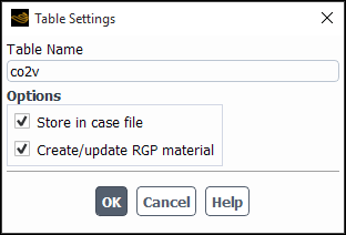
You can use RGP tables to specify the following saturation properties:
Cavitation model: Vaporization Pressure
Evaporation-condensation model: Saturation Temperature
Boiling model: Saturation Temperature
Species-mass-transfer model, Raoult’s law: Saturation Pressure
Phase Interaction Forces: Surface Tension Coefficient (using temperature-dependent values at saturation conditions)
Droplet/Particle evaporation (DPM): Saturation Vapor Pressure
To do this:
Read the RGP table into your case as described in section Reading Files in Tabular Format.
In the dialog box for the selected model, select rgp-table-sat from the drop-down list for the appropriate saturation property.
In the RGP Table Saturation Data dialog box that opens, select the desired saturation table and click .