


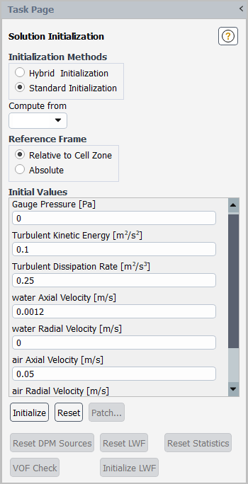
The Solution Initialization task page allows you to define values for flow variables and initialize the flow field to these values. See for details about using this dialog box.
Controls
- Initialization Method
allows you to choose between Hybrid Initialization and Standard Initialization.
- Hybrid Initialization
is a collection of boundary interpolation methods, where variables, such as temperature, turbulence, species fractions, volume fractions, and so on, are automatically patched based on domain averaged values or a particular interpolation recipe (see Hybrid Initialization).
- Standard Initialization
allows you to define values for flow variables and initialize the flow field to these values.
- Compute from
is a drop-down list of zones; the default values for applicable variables will be computed from information contained in the zone that you select from this list. The computation will occur when you select the required zone, and the variable values will be displayed in Initial Values. You can also choose the all-zones item in this list to compute average values based on all zones.
- Reference Frame
indicates whether the initial velocities are absolute velocities (Absolute) or velocities relative to the motion of each cell zone (Relative to Cell Zone). This selection is necessary only if your problem involves moving reference frames or sliding meshes. If there is no zone motion, both options are equivalent.
- Initial Values
displays the initial values of applicable variables. You can use Compute from to compute values from a particular zone, or you can enter values directly. For species transport cases with a single phase flow, only the boundary species that you have selected in the Select Boundary Species dialog box (see Figure 19.3: The Select Boundary Species Dialog Box) appear in the list. You can add or remove a species using the Select Boundary Species dialog box that can be accessed by clicking in the Initialization task page.
initializes the entire flow field to the values listed.
opens the Acoustics Initialization Dialog Box.
resets the fields to their "saved" values.
opens the Patch Dialog Box.
- FMG...
- Species
opens the Select Boundary Species dialog box (see Figure 19.3: The Select Boundary Species Dialog Box), where you can select the boundary species to be displayed in the Initial Values list and in the Patch, Hybrid Initialization, and relevant boundary conditions dialog boxes. You can modify the selected boundary species list on the fly during the problem setup. This item appears for species transport cases with a single phase flow only.
allows you to reset the interphase sources/sinks of momentum, heat, and/or mass to zero. This item is available when you perform coupled discrete phase calculations. See Resetting the Interphase Exchange Terms for details.
- Reset LWF
deletes the Lagrangian wall film (LWF) particles and zeroes out the corresponding face variables without affecting the free stream particles. See Patching the Wall Film for details. This button is available only with the wall-film DPM boundary condition.
can be used to both initialize the flow statistics and reset the flow statistics after you have gathered some data for time statistics. This item is available when you perform unsteady calculations and have enabled the Data Sampling for Time Statistics option in the Run Calculation Task Page. See Inputs for Time-Dependent Problems for details.
- VOF Check
prints a summary report for the VOF case setup. This button is displayed only for VOF multiphase cases. It becomes available after the case is initialized. For details, see Multiphase Case Check.
- Initialize LWF
initializes the Lagrangian wall film (LWF) on all walls with the wall-film DPM boundary condition. This button is available only when the LWF model is used.
opens the Hybrid Initialization Dialog Box. This button is available only when Hybrid Initialization is the selected method.
For additional information, see the following sections:
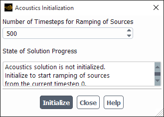
The acoustics initialization dialog box allows you to initialize/reinitialize the solution of the acoustics wave equation and to specify how long to ramp acoustic sources.
Controls
- Number of Timesteps for Ramping of Sources
sets how many timesteps the sound sources will ramp to their full values.
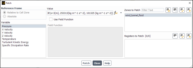
The Patch dialog box allows you to patch different values of flow variables into different cells. See Patching Values in Selected Cells for details about using this feature.
Controls
- Reference Frame
indicates whether patched velocities are absolute velocities (Absolute) or velocities relative to the motion of each cell zone (Relative to Cell Zone). This selection is necessary only if your problem involves moving reference frames or sliding meshes. If there is no zone motion, both options are equivalent. Also, this selection affects only velocities, so the options will not be available unless you have selected a velocity in the Variable list.
- Phase
contains a list of all of the phases in the problem that you have defined. This is available when the VOF, mixture, or Eulerian multiphase model is enabled.
- Variable
contains a list of flow variables from which you can choose the variable to be patched. For species transport cases with a single phase flow, only the boundary species that you have selected in the Select Boundary Species dialog box (see Figure 19.3: The Select Boundary Species Dialog Box) appear in the list. You can add or remove a species using the Select Boundary Species dialog box that can be accessed by clicking in the Initialization task page.
- Volume Fraction Patch Options
contains options that can be used when patching volume fraction for VOF and Eulerian multiphase with Multi-Fluid VOF simulations.
- Patch Reconstructed Interface
applies a piecewise-linear reconstruction of the interface when patching a user-defined register and patches cells that intersect the interface with the actual volume fraction.
- Volumetric Smoothing
enables smoothing of the volume fraction based on the volumetric average over the cell neighbors. After enabling volumetric smoothing, you can click Smooth to apply smoothing to the volume fraction field for all phases in the entire domain.
controls the degree of smoothing applied to the volume fraction field. This can be set between
0(no smoothing) and1(maximum smoothing).
- Value
sets a value to be patched for the selected Variable (constant, by default). Use the drop-down to the right of the field to select either Constant or Expression as the method for specifying the Value.
- Use Field Function
enables the patching of a custom Field Function, rather than a constant Value, for the selected Variable. See Using Field Functions for details.
- Field Function
contains a list of defined custom field functions. If the Use Field Function option is enabled, you can patch one of these functions for the selected Variable. See Using Field Functions for details.
- Zones to Patch
contains a list of cell zones. The specified Value or Field Function for the selected Variable will be patched into the zones you select from this list.
- Registers to Patch
contains a list of cell registers that have been created using the adaption tools. You can patch a different value for a group of cells within a single cell zone by selecting a register containing a subset of the cells in the zone. See Using Registers for details.
updates the flow-field data based on the inputs above.
apply volumetric smoothing to the volume fraction field. This button only appears if is enabled.
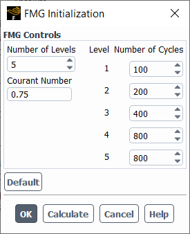
The FMG Initialization dialog box contains the settings that control the Full-Multigrid Initialization strategy.
FMG Controls
- Number of Levels
sets the number of multigrid levels for the FMG iteration (the default is 5).
- Number of Cycles
sets the number of cycles per level. The defaults at each level are 100, 200, 400, 800, and 800.
- Courant Number
sets the FMG iteration Courant-number (the default is 0.75). This will be the CFL value that the FAS multigrid will use for the FMG initialization.
- FMG Options
contains additional FMG customization options supported by the density-based solver (see Additional FMG Initialization Options with the Density-Based Solver).
- Viscous Terms
adds the viscous terms of the Navier-Stokes equation to the FMG initialization procedure.
- Species Reactions
adds the species-reactions terms to the FMG initialization procedure.
- Default
returns the FMG controls to their default values.
The Hybrid Initialization dialog box contains a host of adjustable settings that control the Hybrid Initialization strategy.
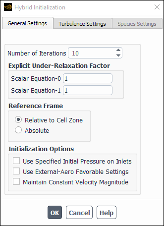
Controls
- General Settings
allow you to adjust such entries as the number of iterations and under-relaxation factors.
- Number of Iterations
uses a default value of 10. This is the number of iterations that will be performed while solving the Laplace equations to initialize the velocity and pressure. If the initialized velocity and pressure fields are not to your liking, you may want to increase the number of iterations and re-initialize the solution.
- Explicit Under-Relaxation Factor
uses a default value of 1. This value will be used while solving the Laplace equation to initialize the velocity and pressure. If the initialized velocity and pressure fields are not to your liking, you may want to adjust the under-relaxation factor and re-initialize the solution.
- Reference Frame
indicates whether the initial velocities are absolute velocities (Absolute) or velocities relative to the motion of each cell zone (Relative to Cell Zone). This selection is necessary only if your problem involves moving reference frames or sliding meshes. If there is no zone motion, both options are equivalent.
- Initialization Options
allows you to include any of the three initialization options.
- Use Specified Initial Pressure on Inlets
if you want the specified pressure for Supersonic/Initialization Gauge Pressure at the inlet boundaries to be used for solving the Laplace equation for the pressure.
- Use External-Aero Favorable Settings
if you want to have the velocity potential patched with a linear value to help accelerate convergence of Scalar Equation–0 and to obtain a better guess of the velocity field for external-aero problems.
- Maintain Constant Velocity Magnitude
if you want to use the flow direction obtained from solving the velocity potential (Scalar Equation–0), while maintaining a constant velocity magnitude throughout the computational domain.
- Turbulence Settings
uses by default the domain averaged values for the turbulence parameters. If you want to use variable turbulence parameters you can deselect the Average Turbulent Parameters check box. When this option is disabled, then it calculates the turbulent parameters, such as kinetic energy, dissipation energy, and so on, using local flow parameters.
- Species Settings
will by default initialize secondary species with zero mass or mole fractions. If you want to specify the appropriate value for the species, you must enable Specify Species Parameters. Note that only the boundary species that you have selected in he Select Boundary Species dialog box (see Figure 19.3: The Select Boundary Species Dialog Box) appear in the list. You can add or remove a species using the Select Boundary Species dialog box that can be accessed by clicking in the Initialization task page.