


Important: Double Precision is recommended for all multiphase cases.
The following topics are discussed:
General strategies that are applicable to multiphase models are discussed in the following sections:
- 26.8.1.1. Coupled Solution for Eulerian Multiphase Flows
- 26.8.1.2. Coupled Solution for VOF and Mixture Multiphase Flows
- 26.8.1.3. Selecting the Pressure-Velocity Coupling Method
- 26.8.1.4. Controlling the Volume Fraction Coupled Solution
- 26.8.1.5. Default and Stability Controls
- 26.8.1.6. Heat Transfer and Radiative Flux Distribution for Non-Eulerian Multiphase Models
- 26.8.1.7. Steady-State Solution Strategies
In multiphase flow, the phasic momentum equations, the shared pressure, and the phasic volume fraction equations are highly coupled. Traditionally, these equations have been solved in a segregated fashion using some variation of the SIMPLE algorithm to couple the shared pressure with the momentum equations. This is attained by effectively transforming the total continuity into a shared pressure. The Ansys Fluent Phase Coupled SIMPLE algorithm has been successfully implemented and solves a wide range of multiphase flows. However, coupling the linearized system of equations in an implicit manner would offer a more robust alternative to the segregated approach.
One of the fundamental problems is that the resulting matrix is not symmetric and that the continuity constraint may contribute to a zero diagonal block, making the solution difficult to obtain. One way to circumvent this problem is to use direct solvers, but these are too expensive for large industrial cases. In addition, we need to avoid a zero diagonal, resulting from the continuity constraint, and like the segregated solver, we need to construct a pressure correction equation. In multiphase, we also have the additional problem of the vanishing phase, which for the coupled solver is important to ensure some continuity in the coefficients. Like the Phase Coupled, we use a Rhie and Chow type of scheme to calculate volume fluxes and to provide proper coupling between velocity and pressure, thereby avoiding unphysical oscillations.
Consider a single-phase system and let us denote the velocity correction components in
the three Cartesian directions by  ,
,  , and
, and  with
with  denoting the shared pressure correction. These are discrete variables
and can be expressed in the form
denoting the shared pressure correction. These are discrete variables
and can be expressed in the form  . The linear system that is generated by the single-phase coupled solver
is of the form
. The linear system that is generated by the single-phase coupled solver
is of the form
 | (26–34) |
For a notation in component form 
 | (26–35) |
Now let us consider a multiphase system of n-phases and denote the phasic velocity
correction components in the three Cartesian directions by  ,
,  , and
, and  where the subscript
  represents the phase notation,
  denotes the shared pressure correction and
  denotes the volume fraction correction (Ansys Fluent can solve in both
correction form for velocity and volume fraction and non-correction form). For simplicity
the matrix will be shown for two phases. The vector solution is of the form
denotes the volume fraction correction (Ansys Fluent can solve in both
correction form for velocity and volume fraction and non-correction form). For simplicity
the matrix will be shown for two phases. The vector solution is of the form
 or in a shorter notation
  . The linear system would be an extension of the one generated by the
coupled solver shown by Equation 26–34.
. The linear system would be an extension of the one generated by the
coupled solver shown by Equation 26–34.
 | (26–36) |
This system can be easily generalized to  phases. The components of this matrix are also matrices.
For large problems, we need to resort to iterative solvers. The Ansys Fluent AMG Coupled solver with an ILU smoother has proved to be a robust method. Most coupled solvers also need a pseudo stepping method, adding more diagonal dominance to the matrix. Our method here is to use under-relaxation factors for momentum, which is equivalent to time stepping in steady flows. Similar to that of the single phase, we have introduced a steady Courant Number instead of an under-relaxation for velocities. Having this control is important when using second order numerical schemes in the convective terms.
For the sake of simplicity, input parameters for the Coupled solver are similar to the single-phase solver. We have the options for solving the whole system including volume fraction, or to treat the volume fraction solution in a segregated manner while preserving the pressure-velocity coupling for all phases.
Important: Equations in multiphase are more strongly linked than single phase and generally may need more under-relaxation, hence using the same values as single phase may not be ideal. A low Courant number would stabilize the solution.
See Selecting the Pressure-Velocity Coupling Method for information about applying the various algorithms.
We have the option of solving the multiphase system for VOF and mixture multiphase models in the following ways:
Solving the continuity and momentum equations in a coupled manner (see Coupled Algorithm in the Theory Guide) and solving the volume fraction equation in a segregated manner.
Solving the volume fraction equation in a coupled manner along with the continuity and momentum equations.
Solving the volume fraction equation in a coupled manner requires discretization of the volume fraction equation in the correction form along with the discretization of the continuity and momentum equation, as discussed in Coupled Algorithm in the Theory Guide.
The volume fraction equation could be represented in the discretized form as
 | (26–37) |
The overall system of equations after being transformed to the correction form could be represented as
 | (26–38) |
For a 2D case and two-phase flow, the system could be expanded as follows:
 | (26–39) |
and the unknown and residual vectors have the form
 | (26–40) |
 | (26–41) |
| where | |
 = coefficient matrix = coefficient matrix | |
 = solution vector = solution vector | |
 = residual vector = residual vector | |
 = pressure correction = pressure correction | |
 = velocity corrections = velocity corrections | |
 = volume fraction correction = volume fraction correction |
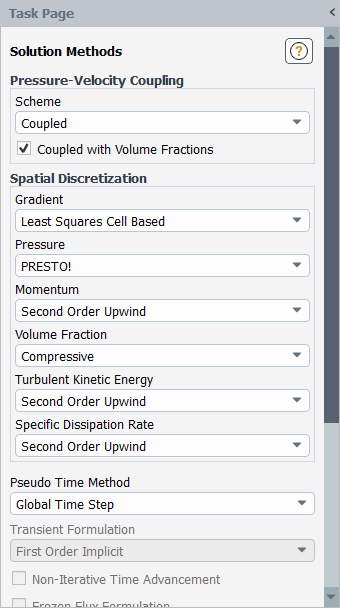
The settings that are available in the Solution Methods task page (see Figure 26.113: The Solution Methods Task Page Displaying The Pressure-Velocity Coupling Options) for solving the coupled system of equations arising in multiphase flows are:
- Schemes
Phase Coupled SIMPLE (Eulerian multiphase)
PISO (VOF and mixture)
SIMPLE (VOF and mixture)
SIMPLEC (VOF and mixture)
Coupled (all multiphase models)
- Options
Coupled with Volume Fractions (all multiphase models except the mixture model with the Slip Velocity option and the wet steam model)
Solve N-Phase Volume Fraction Equations (mixture and Eulerian models)
The PISO, SIMPLE, and SIMPLEC schemes apply to the VOF and mixture models and are discussed in Pressure-Velocity Coupling in the Theory Guide.
The Phase Coupled SIMPLE (PC-SIMPLE) is an extension of the SIMPLE algorithm [114] to multiphase flows. The velocities are solved coupled by phases in a segregated fashion. Fluxes are reconstructed at the faces of the control volume and then a pressure correction equation is built based on total continuity. The coefficients of the pressure correction equations come from the coupled per phase momentum equations. This method has proven to be robust and it is the only method available for all previous versions of Ansys Fluent.
The Coupled scheme (also known as Multiphase Coupled in previous Ansys Fluent versions) solves all equations for phase velocity corrections and shared pressure correction simultaneously [50]. These methods incorporate the lift forces and the mass transfer terms implicitly into the general matrix. This method works very efficiently in steady-state situations, or for transient problems when a larger time step size is required.
The Coupled with Volume Fractions option (also known as Full Multiphase Coupled in previous Ansys Fluent versions) couples velocity corrections, shared pressure corrections, and the correction for volume fraction simultaneously. Theoretically, it should be more efficient, however it may have some drawbacks in robustness and CPU time usage. The robustness issue stems from the lack of control of the solution of the volume fraction equation. The continuity constraint (sum of all volume fractions equals 1, and individual values limited between zero and one) cannot be enforced exactly during inner solver iterations, and slight variations from the physical limits may lead to divergence. Research is ongoing in this area to improve the method. The method is advantageous for heterogeneous mass transfer when a low Courant number is given; it also works well in dilute situations.
The Volume Fraction Coupling Method aims to achieve a faster steady-state solution compared to the segregated method of solving equations. It may not be a suitable option for transient applications due to the significant overhead in CPU time compared to the segregated method, unless it is run with a larger time step size.
Note: The Coupled with Volume Fractions option is available in the interface after you have selected Coupled from the Scheme drop-down list for Pressure-Velocity Coupling. For steady-state cases, Global Time Step will be automatically selected from the Pseudo Time Method list when you enable the Coupled with Volume Fractions option for the VOF and mixture models.
The coupled with volume fractions option has the following limitations:
It is not available when Slip Velocity is enabled for the Mixture multiphase model.
It is not supported when using the Singhal-Et-Al cavitation model.
It is not supported when the Explicit formulation for volume fraction is selected.
Recommended uses of the coupled with volume fractions option:
Selecting global time step for the pseudo time method is recommended for steady-state calculations.
It is recommended that you use lower under-relaxation factors for momentum for higher order schemes.
For marine applications, it is recommended that you use a low-order variant or hybrid treatment for the Rhie-chow face flux interpolation (see High-Order Rhie-Chow Face Flux Interpolation).
For a multiphase flow, the sum of the phase volume fractions must always equal 1. By default, Fluent enforces this constraint by solving the volume fraction equations for each of the secondary phases and then setting the volume fraction of the primary phase to the complement.
In certain cases, where poor convergence and/or mass imbalance are observed, enabling Solve N-Phase Volume Fraction Equations may improve solutions, although in practice the results obtained from using this option are case dependent. If selected, this option will solve all volume fraction equations, including both primary and secondary phases. The resulting phase volume fractions are then scaled in order to satisfy the requirement of summing to 1. This approach is more computationally expensive than the default approach and, in general, should not be necessary for the simulation.
Note: The Solve N-Phase Volume Fraction Equations option is not available for the Volume of Fluid model or Eulerian with Multi-Fluid VOF Model enabled.
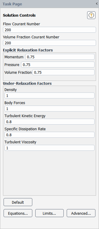
When using the Coupled with Volume Fractions scheme, you will need to specify the following in the Solution Controls task page (see Figure 26.114: The Solution Controls Task Page Displaying the Coupled Volume Fraction Method for the VOF and Mixture Models):
VOF and Mixture Multiphase Model:
For steady-state cases using a pseudo time method (global time step), specify the Volume Fraction Courant Number, and the Pseudo Time Explicit Relaxation Factors. The Pseudo Time Explicit Relaxation Factors are described in Global Time Step Method Settings.
Note: The Pseudo Time Explicit Relaxation Factors for the Volume Fraction is set to 0.5 by default.
For transient cases or steady-state cases with the pseudo time method turned off, enter the Flow Courant Number, the Volume Fraction Courant Number, Explicit Relaxation Factors, and the Under-Relaxation Factors.
Note: By default, the Volume Fraction is set to 0.75 for transient cases and 0.5 for steady-state cases in the Explicit Relaxation Factors group box.
Figure 26.114: The Solution Controls Task Page Displaying the Coupled Volume Fraction Method for the VOF and Mixture Models
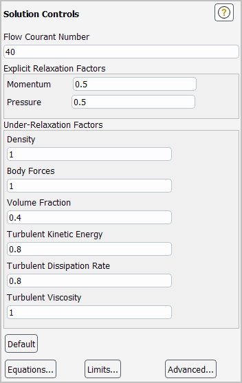
Eulerian Multiphase Model:
For steady-state cases using a pseudo time method (global time step), specify the Pseudo Time Explicit Relaxation Factors as described in Global Time Step Method Settings.
Note: The Pseudo Time Explicit Relaxation Factors for the Volume Fraction is set to 0.5 by default.
For transient cases or steady-state cases with the pseudo time method turned off, enter the Flow Courant Number, the Explicit Relaxation Factors, and the Under-Relaxation Factors.
Note: The under-relaxation for Volume Fraction is set by using an implicit Under-Relaxation Factor, rather than a Volume Fraction Courant Number, and is 0.5 by default.
Figure 26.115: The Solution Controls Task Page Displaying the Coupled Volume Fraction Method for the Eulerian Multiphase Model
Ansys Fluent provides you with the tools to manage the version-specific defaults.
Starting from version 2020-R1, for newly created cases, the new multiphase defaults will be applied automatically. If you read in an old case file saved in any version prior to Ansys Fluent 2020 R1, the existing settings will be respected.
If you want to apply the new multiphase defaults to the pre 2020-R1 case, you can issue the text user interface (TUI) command as shown in the example below. The information about the new settings will be printed in the Ansys Fluent console. You can review these settings prior to executing the changes.
solve/set/multiphase-numerics/default-controls/
recommended-defaults-for-existing-cases

The multiphase flow default changes integrated in Fluent version 2020-R1 are
as follows:
 Operating Conditions :
  - In case of gravity, the operating density method is changed to minimum
    of phase averaged densities.
 Surface Tension :
 - For surface tension force modeling, the number of smoothings for volume
   fraction is changed to 2.
 Initialization :
 - The Patch Reconstructed Interface and Volumetric Smoothing options are
   enabled.
 - The Volumetric Smooting Relaxation Factor is changed to 0.5.
 - These settings are applied when executing the Patch and Smooth commands.
 Solver Methods :
 - The unstructured variant of PRESTO is enforced irrespective of a mesh type.

Do you want to execute these default changes? [no] yes
To revert some of the new defaults to the pre-R20.1 default settings, you can use the text commands shown in the example below:
Revert to the old default of operating density method? [no]yes- the operating density method has changed to mixture-averaged. Revert to the old default of volume fraction smoothings for surface tension? [no]yes- the number of volume fraction smoothings has changed to 1. Revert to the old variant of PRESTO for cases using structured mesh? [no]yes- the structured variant of PRESTO has been enabled for structured mesh.
The VOF model is numerically more challenging compared to other models due to resolution of sharp discontinuities in the flow system. Body force and pressure gradient imbalances near free surface may lead to unphysical acceleration of the lighter phase. Diffusing these discontinuities adversely affects the interface accuracy; therefore, it may not be an efficient approach.
Complex VOF applications may also suffer from solution instabilities due to several other reasons:
Improper settings
Too large time step size
Higher order oscillations
Improper convergence
Poor mesh
Meshing events where interpolated quantities do not satisfy continuity
Ansys Fluent offers the following options for controlling the solution process:
Stabilization methods
Velocity limiting treatment
To access the stabilization methods:
In the Solution Methods task page, click the button (VOF Solution Stability Controls group box).
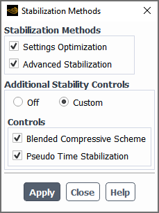
In the Stabilization Methods dialog box that opens, you can enable the following methods:
- Settings Optimization
makes the basic optimization changes in the case setup depending on the type of physics to promote better stability.
- Advanced Stabilization
enables advanced numerical methods and treatments that are important for solution stability. You can use this option as a first step to improve solution stability without significantly compromising its accuracy.
- Additional Stabilization Controls
contains controls that facilitates better solution stability with aggressive settings by adding diffusion in space and time (Off by default). You can use this option as a second step of solution stabilization. When Custom is selected, you can enable the following option:
- Blended Compressive Scheme
applies the following settings:
Sharp/Dispersed interface modeling type
Compressive volume fraction spatial discretization
Slope limiter = 1.5
- Pseudo Time Stabilization
uses the following methods:
False time stepping
This method provides additional stability for buoyancy-driven flows in the steady-state pseudo time method mode by increasing the diagonal dominance using the false time step size.
Momentum stabilization
This item is available only for the steady-state solver.
Pseudo time stabilization options are available via the Text User Interface (TUI) as described in Text User Interface for VOF Stability Controls.
To access the velocity limiting treatment:
In the Solution Methods task page, click the button (VOF Solution Stability Controls group box).
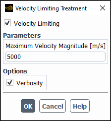
In the Velocity Limiting Treatment dialog box that opens, enable Velocity Limiting.
Unphysical velocity spikes may arise from solution instabilities. Most often, the velocity spikes are very local in nature and subside as the iterations progress. However, sometimes these spikes may grow and can cause sudden divergence. The velocity limiting treatment can increase the solution stability by curbing these spikes, which are numerical and local in nature.
In the Parameters group box, you can adjust the Maximum Velocity Magnitude.
This limit can be roughly taken as 2-3 times of system bulk velocity.
If you want the number of cells where the limiting is applied to be printed every time-step, enable Verbosity. Note that excessive limiting can adversely affect the convergence and may pose a question on the validity of results.
The solution stabilization controls can be also set in the Text User Interface (TUI). The TUI also provides additional options.
Additional stabilization controls can be executed using the following text commands:
solve/set/multiphase-numerics/solution-stabilization/execute-additional-stability-controls?solve/set/multiphase-numerics/solution-stabilization/execute-advanced-stabilization?solve/set/multiphase-numerics/solution-stabilization/additional-stabilization-controls/execute-settings-optimization?
For complex VOF and mixture multiphase cases, Ansys Fluent provides advanced options for improving stability via the following text commands:
solve/set/multiphase-numerics/advanced-stability-controls/The available controls are:
Pseudo time stability controls
These controls are available for the Coupled pressure-velocity coupling scheme with Global Time Step selected from the Pseudo Time Method list. They can be accessed via the
solve/set/multiphase-numerics/advanced-stability-controls/pseudo-time/TUI menu:You can use the following options:
-
solve/set/multiphase-numerics/advanced-stability-controls/pseudo-time/false-time-step-linearization? Provides additional stability for buoyancy-driven flows in the steady-state pseudo time method mode by increasing the diagonal dominance using the false time step size.
-
solve/set/multiphase-numerics/advanced-stability-controls/pseudo-time/smoothed-density-stabilization-method? Smooths the cell density near the interface, therefore avoiding unphysical acceleration of lighter phase in the vicinity of interface. The default number of density smoothings is 2. In case of very large unphysical velocities across the interface, you can increase this number when prompted with
Number of density
                          smoothings
.
For automatic pseudo time step calculations, you can use the advanced method for better solution stability. The method is available only when the Automatic time step method is used for a pseudo time step calculation (see Pseudo Time Settings for the Calculation for details). It is enabled by issuing the following text command:
solve/set/multiphase-numerics/advanced-stability-controls/pseudo-time/auto-dt-advanced-controls/enable?Enable advanced automatic time-stepping? [no]yesIn addition to time scales described in Global Time Step Method in the Fluent Theory Guide, this method considers viscous and surface tension time scales using the following correlations.

(26–42)

(26–43)
In Equation 26–42 and Equation 26–43, the following nomenclature is used:
 = viscous time scale
 = surface tension time scale
 = length scale based on the user-selected method
 = averaged kinematic viscosity
 = averaged fluid density
 = surface tension coefficient
You can use the following controls available via the TUI to adjust the advanced method settings:
solve/set/multiphase-numerics/advanced-stability-controls/pseudo-time/auto-dt-advanced-controls/dt-factor-maxSets the maximum limit for increasing the size of the pseudo time step. Default: 1.2.
solve/set/multiphase-numerics/advanced-stability-controls/pseudo-time/auto-dt-advanced-controls/dt-factor-minSets the minimum limit for increasing the pseudo time step size. Default: 0.25.
solve/set/multiphase-numerics/advanced-stability-controls/pseudo-time/auto-dt-advanced-controls/dt-init-limitSets the maximum pseudo time step size for the first iteration. Default: 0.01s.
The time step size during the first iteration may not be optimal due to lack of solution data or time-step estimation methods for all possible scenarios. A very large time step size at the start can distort the whole solution; therefore, limiting the initial time step size can help to smooth the start of the simulation.
solve/set/multiphase-numerics/advanced-stability-controls/pseudo-time/auto-dt-advanced-controls/dt-maxSets the maximum pseudo time step size for the entire simulation. Default: 1000s.
solve/set/multiphase-numerics/advanced-stability-controls/pseudo-time/auto-dt-advanced-controls/max-velocity-ratioSets the maximum velocity ratio (maximum velocity to average velocity) above which the solver freezes the time step size for better solution stability. Default: 100.
Note: Since the predicted time step size depends heavily on the length scale, you should specify a representative Length Scale Method (in the Run Calculation task page, Pseudo Time Settings group box) based on your problem.
-
Equation order controls
These controls are accessed via the
solve/set/multiphase-numerics/advanced-stability-controls/equation-order/TUI menu.By default, Ansys Fluent solves the flow at the start of each iteration (except for explicit VOF problems where the flow is solved right after solving the volume fraction equation). You can use the
solve-flow-last?text option (under theequation-orderTUI menu) to solve the flow equation at the end of each iteration. This may improve the behavior at the start of the new time step if the solution does not converge properly.Pressure velocity coupling controls
These controls are accessed via the
solve/set/multiphase-numerics/advanced-stability-controls/p-v-coupling/TUI menuThe following options are available:
coupled-vof/By default, Ansys Fluent performs the linearization of the buoyancy terms with respect to the volume fraction while solving the momentum equation. This is critical for fast convergence. However, for certain unstable cases, using the linearization in all regions except near the free surface (the blended treatment of the buoyancy force linearization) may provide better stability. This can be done via the
buoyancy-force-linearization?text command (under thecoupled-vof/TUI menu).pressure-interpolation/You can use the modified variant of the Body Force Weighted pressure interpolation scheme for improved robustness and convergence behavior in general. This option is available via the
modified-bfw-schemetext commend and is highly recommended for flows with a high viscosity ratio where the original body force weighted scheme has severe limitations. Note that this scheme may not offer the same level of accuracy for very highly rotating flows as PRESTO.rhie-chow-flux/For collocated grids, an accurate calculation of flux at the cell faces is extremely important in order to avoid pressure and velocity checkerboarding. However, sometimes higher-order interpolations become a source of instability in the vicinity of free surface or for a highly-skewed mesh. If the solution becomes unstable while using the higher-order momentum discretization, try switching to the low-order flux calculation (rather than the low-order momentum discretization) by using the
low-order-rhie-chow?text option (under therhie-chow-fluxTUI menu). This option uses the low-order velocity interpolation in the flux calculation.skewness-correction/You can use the
limit-pressure-correction-gradient?option (under theskewness-correction/TUI menu) to limit the pressure correction gradient term for better stability on a skewed mesh while using skewness corrections with the PISO, SIMPLEC, or Fractional-Step pressure-velocity coupling scheme.
For Eulerian multiphase models, the energy equation is solved in the phase domain and therefore, heat flux can be reported based on the mixture domain or any of the phases individually. However, for the VOF and Mixture multiphase models, the energy equation is discretized in the phase domains but solved only in the Mixture domain after summing over the individual phases. Boundary heat fluxes for flow boundaries are stored at the phase domain but wall heat fluxes are only stored at the mixture domain. This approach of modeling wall heat fluxes using mixture domain properties has certain deficiencies in proper accounting and reporting of phasic wall heat fluxes.
The phasic wall heat fluxes for the VOF and Mixture multiphase models can be calculated using an approach which makes use of the linearized coefficients at the phase level. These coefficients are then accumulated in the mixture domain to be used in the energy equation. This phasic approach corrects the reporting of wall heat fluxes at the wall boundaries.
The phasic approach can activated using the following text command:
/solve/set/multiphase-numerics/energy/phasic-wall-heat-flux-form?
Note that the default is no meaning the phasic formulation is
not used. To enable, respond yes to the prompt, and then you may
initialize or continue the run with the phasic formulation active.
For steady-state problems that either involve a closed domain or have no separate inflow/outflow boundaries for all the phases, mass conservation cannot be guaranteed with the pseudo time method set to global time step. It might be better to run these problems with the transient solver using few iterations per time step to achieve faster results.
Strategies that are applicable to specific multiphase models are discussed in the following sections:
Several recommendations for improving the accuracy and convergence of the VOF solution are presented here.
The site of the reference pressure can be moved to a location that will result in less round-off in the pressure calculation. By default, the reference pressure location is the center of the cell at or closest to the point (0,0,0). You can move this location by specifying a new Reference Pressure Location in the Operating Conditions Dialog Box.
![]() Setup →
Setup → ![]() Cell Zone
Conditions → Operating Conditions...
Cell Zone
Conditions → Operating Conditions...
The position that you choose should be in a region that will always contain the least dense of the fluids (for example, the gas phase, if you have a gas phase and one or more liquid phases). This is because variations in the static pressure are larger in a more dense fluid than in a less dense fluid, given the same velocity distribution. If the zero of the relative pressure field is in a region where the pressure variations are small, less round-off will occur than if the variations occur in a field of large nonzero values. Thus in systems containing air and water, for example, it is important that the reference pressure location be in the portion of the domain filled with air rather than that filled with water.
For all VOF calculations, you should use the body-force-weighted pressure interpolation scheme or the PRESTO! scheme.
![]() Solution →
Solution → ![]() Controls
Controls
By default, Ansys Fluent uses an unstructured variant of the PRESTO pressure scheme for all types of meshes. For cases created in versions prior to Ansys Fluent 2020 R1, the structured variant of the PRESTO scheme will be used for structured meshes.
To enable the unstructured variant of the PRESTO scheme, use the following text command:
solve/set/vof-numerics
When prompted with
Use unstructured variant of PRESTO pressure scheme?
            [no]
Answer yes.
Note: You do not need to use this text command option for cases that involve unstructured meshes since the unstructured variant of the PRESTO scheme is automatically enabled for such cases.
The availability of discretization schemes for volume fraction is summarized in Spatial Discretization Schemes for Volume Fraction.
If you are modeling a sharp interface regime on meshes that have high aspect ratio cells, large jumps in cell size, or high skewness, interface capturing schemes such as Compressive and CICSAM will not produce very sharp results. For such cases, you should use the Geo-Reconstruct scheme.
For meshes of good quality, it is recommended that you use the Compressive scheme, which is available in both explicit and implicit formulations and is applicable to both sharp and dispersed flow regimes. The Compressive scheme also provides better accuracy compared with CICSAM and Modified HRIC for most cases. When used with the implicit formulation and the second order time scheme, the Compressive scheme produces quite a sharp interface.
When using the Compressive spatial discretization scheme, it is recommended that you use step-wise sharpening after the flow transitions from the diffused zone to the sharpening zone. In other words, you would want to transition from first order to second order, followed by a transition from second order to compressive. You would want to take this approach if the flow has a smooth transition from a sharp interfacial zone to a diffused interfacial zone. However, if the flow has a nonuniform transition from a diffused interfacial zone to a sharp interfacial zone, this might create unphysical sharpening of the interface if not handled properly, especially for transient cases. For example, transitioning from a slope limiter of 2 (compressive) to a slope limiter of 0 or 1 (first order or second order) might be acceptable, but a first order to compressive transition might create unphysical sharpening of the interface.
If you are solving a problem with the evaporation-condensation mass transfer mechanism enabled (Including Mass Transfer Effects) it is recommended that you use one of the diffusive interface capturing schemes such as QUICK, HRIC, or Phase Localized Compressive (Discretizing Using the Phase Localized Compressive Scheme).
Important: The BGM scheme produces a sharp interface, which may result in poor convergence in some cases. In such situations, we recommend you use a low value for the VOF under-relaxation. In addition, you can start with the Compressive or Modified HRIC scheme and then switch to the BGM scheme.
In VOF modeling, using a high-order discretization scheme for the momentum transport equations may reduce the stability of the solution compared to cases using first-order discretization. In such situations, there are a couple of recommendations:
Use a low-order variant of the Rhie-Chow face flux interpolation. This is enabled using the following text command:
solve→set→numericsYou will be asked
disable high order Rhie-Chow flux? [no]
to which you will respond
yes.Use a hybrid treatment of high-order Rhie-Chow face flux interpolation. This is enabled using the following text command:
solve→set→vof-numericsYou will be asked
Use hybrid treatment for high order Rhie-Chow flux? [no]
to which you will respond
yes.Hybrid treatment allows you to use a high-order variant of the Rhie-Chow face flux interpolation everywhere inside the domain, except in the vicinity of the interface where a low-order variant is used for the interpolation of the face flux. This treatment could be helpful to get better convergence without compromising much of the accuracy.
For cases using Moving Mesh/Dynamic Mesh/Multiple Reference Frame models, Ansys Fluent does not consider the unsteady terms for Rhie-Chow face flux interpolation by default. Accounting for the unsteady terms helps to achieve better solution stability, especially when using a lower time step size with the PRESTO scheme.
To enable forced treatment of unsteady terms in Rhie-Chow face flux interpolation, use the following text command:
solve → set →
vof-numerics
You will be asked
Use forced treatment of unsteady terms in Rhie-Chow flux? [no]
to which you will respond yes.
Another change that you should make to the solver settings is in the pressure-velocity coupling scheme and under-relaxation factors that you use. The PISO scheme is recommended for transient calculations in general. Using PISO allows for increased values on all under-relaxation factors, without a loss of solution stability. You can generally increase the under-relaxation factors for all variables to 1 and expect stability and a rapid rate of convergence (in the form of few iterations required per time step). For calculations on tetrahedral or triangular meshes, an under-relaxation factor of 0.7–0.8 for pressure is recommended for improved stability with the PISO scheme.
![]() Solution →
Solution → ![]() Controls
Controls
As with any Ansys Fluent simulation, the under-relaxation factors will need to be decreased if the solution exhibits unstable, divergent behavior with the under-relaxation factors set to 1. Reducing the time step size is another way to improve the stability.
You should begin the mixture calculation with a low under-relaxation factor for the slip velocity. A value of 0.2 or less is recommended. If the solution shows good convergence behavior, you can increase this value gradually.
For some cases (for example, cyclone separation), you may be able to obtain a solution more quickly if you compute an initial solution without solving the volume fraction and slip velocity equations. Once you have set up the mixture model, you can temporarily disable these equations and compute an initial solution.
![]() Solution →
Solution → ![]() Controls
Controls
In the Equations Dialog Box, deselect Volume Fraction and Slip Velocity in the Equations list. You can then compute the initial flow field. Once a converged flow field is obtained, turn the Volume Fraction and Slip Velocity equations back on again, and compute the mixture solution.
To improve convergence behavior, you may want to compute an initial solution before solving the complete Eulerian multiphase model. There are multiple methods you can use to obtain an initial solution for an Eulerian multiphase calculation:
Set up and solve the problem using the mixture model (with slip velocities) instead of the Eulerian model. You can then enable the Eulerian model, complete the setup, and continue the calculation using the mixture-model solution as a starting point.
Set up the Eulerian multiphase calculation as usual, but compute the flow for only the primary phase. To do this, deselect Volume Fraction in the Equations list in the Equations Dialog Box. Once you have obtained an initial solution for the primary phase, turn the volume fraction equations back on and continue the calculation for all phases.
Use the mass-flow inlet boundary condition to initialize the flow conditions. It is recommended that you set the value of the volume fraction close to the value of the volume fraction at the inlet.
At the beginning of the solution, a smaller time step size is recommended in order to reach convergence.
If using the volume fraction explicit scheme, do not start with a large Courant number at the beginning of your run.
If using the volume fraction explicit scheme, start a run with a smaller time step size and then increase it. Alternatively, this could be done by using multiphase-specific time stepping, which would increase the time step size based on the input parameters.
For problems involving a free surface or sharp interfaces between the phases, using the symmetric drag law (available in the Forces tab of the Multiphase Model dialog box) is recommended.
Multiphase-specific time stepping is not recommended for compressible flows.
Important: You should not try to use a single-phase solution obtained without the mixture or Eulerian model as a starting point for an Eulerian multiphase calculation. Doing so will not improve convergence, and may make it even more difficult for the flow to converge.
If you are planning to include the effects of lift and/or virtual mass forces in a steady-state Eulerian multiphase simulation, you can often reduce stability problems that sometimes occur in the early stages of the calculation by temporarily ignoring the action of the lift and the virtual mass forces. Once the solution without these forces starts to converge, you can interrupt the calculation, define these forces appropriately, and continue the calculation.
For problems involving a packed-bed granular phase with very small particle sizes
(on the order of 10  m), convergence can be obtained by using the W-cycle multigrid for the
pressure. In the Multigrid tab, under Fixed Cycle
Parameters in the Advanced Solution Controls Dialog Box, you
may need to use higher values for Pre-Sweeps,
Post-Sweeps, and Max Cycles. When you are
choosing the values for these parameters, you should also increase the
Verbosity to
m), convergence can be obtained by using the W-cycle multigrid for the
pressure. In the Multigrid tab, under Fixed Cycle
Parameters in the Advanced Solution Controls Dialog Box, you
may need to use higher values for Pre-Sweeps,
Post-Sweeps, and Max Cycles. When you are
choosing the values for these parameters, you should also increase the
Verbosity to 1 in order to monitor the
AMG performance; that is, to make sure that the pressure equation is solved to a desired
level of convergence within the AMG solver during each global iteration. See Defining the Phases for the Eulerian Model for more information about granular
phases, and The V and W Cycles in the Theory Guide and Modifying Algebraic Multigrid Parameters for details about multigrid cycles.
When using the anisotropic drag law (Including the Multi-Fluid VOF Model), it is recommended that you start the solution with a lower anisotropy ratio. After your solution has run for some time, you can then increase the ratio by reducing the friction factor in the tangential direction. Note that You can also start the solution with the symmetric drag law, then change to the anisotropic drag law.
Using a smaller under-relaxation for pressure and momentum may also help in convergence for cases with a higher anisotropy ratio.
If the flow for a particular phase is important in both directions (normal and
tangential to the interface), use a lower anisotropy ratio, between 100-1000. A higher
anisotropy ratio might cause an unstable solution for such cases. For a higher
anisotropy ratio of more than 1000, a smaller under-relaxation for pressure and momentum
is recommended. When using the coupled multiphase solver, if the solution is unstable
with a higher anisotropy ratio, then reducing the courant number may be beneficial.
Anisotropic Drag Method [1], with Viscosity
option [2] is recommended for a higher viscosity ratio.
In the Eulerian multiphase model, the volume fraction and continuity equations (see Equation 14–203 in the Fluent Theory Guide) can be represented either in the mass or volumetric form by choosing a reference density method using the following text command:
solve/set/mp-reference-density
The available reference methods are listed in the below table.
| Reference Density Method | Volume Fraction Equation Representation | Continuity Equation Representation | Phase Reference Density Calculation |
|---|---|---|---|
0 (default) | Mass form | Volumetric form | Averaged density of the phase |
1 | Mass form | Volumetric form | Cell density of the phase |
2 | Mass form | Mass form | 1 |
3 | Volumetric form | Volumetric form | Cell density of the phase |
There is not much difference between Methods 0 and
1 for incompressible flows. Method
2, in general, may not be very stable at larger time steps and,
therefore, is not recommended. Method 3 is similar to the
Mixture multiphase model and may provide better stability in certain cases.
Note that both the volume fraction and continuity equations remain mass conservative regardless of their representation. Different representations affect only the solution stability and convergence behavior.
For the Eulerian multiphase model, the Non-Iterative Time Advancement (NITA) scheme uses PISO as a pressure velocity coupling method, where the pressure correction equation is solved in two steps named predictor and corrector.
For the face pressure calculation, the Eulerian multiphase model uses PRESTO as a default method for both the predictor and corrector steps.
You can change the face pressure interpolation method using the following text command:
solve/set/multiphase-numerics/nita-controls/face-pressure-options
To select Body Force Weighted as a face pressure interpolation method for both
predictor and corrector steps, enter
at the yes
enable body-force-weighted for face pressure
              calculation?
prompt.
To select the Second Order method as a face pressure interpolation method for both predictor and corrector steps:
Enter
noenable body-force-weighted for face pressure calculation?prompt.When prompted with
face pressure calculation method for predictor
                  step
, choose Second Order (1
To select the Second Order method as a face pressure interpolation method for the corrector step only:
Enter
noenable body-force-weighted for face pressure calculation?prompt.When prompted with
face pressure calculation method for predictor
                  step
, retain the default selection of PRESTO (0When prompted with
face pressure calculation method for corrector
                  step
, choose Second Order (1
When PRESTO is used for the face pressure calculation, you
will be asked whether you want to exclude transient terms. Because the impact of fluxes
on the face pressure is inversely proportional to the time step size, which may lead to
numerical problems as the time step size decreases, the exclusion of transient terms is
recommended for very small time steps when using PRESTO:
exclude transient terms in face pressure calculation? [no]
                yes
When you use the wet steam model (described in Wet Steam Model Theory in the Theory Guide, and Setting Up the Wet Steam Model), the following two field variables will show up in the inflow, outflow boundary dialog boxes, and in the Solution Initialization task page and Patch dialog boxes.
Liquid Mass Fraction (or the wetness factor)
In general, for dry steam entering flow boundaries the wetness factor is zero.
Log10 (Droplets Per Unit Volume)
In general this value is set to zero, indicating zero droplets entering the domain.
When you select the wet steam model for the first time, a message is displayed indicating that the Minimum Static Temperature should be adjusted to 273 K since the accuracy of the built-in steam data is not guaranteed below a value of 273 K. If you use your own steam property functions, you can adjust this limit to whatever is permissible for your data.
To adjust the temperature limits, go to the Solution Limits dialog box.
![]() Solution
→ Controls
Solution
→ Controls![]() Limits...
Limits...
The default maximum wetness factor or liquid mass fraction ( ) is set to 0.1. In general, during the convergence process, it is
common that this limit will be reached, but eventually the wetness factor will drop
below the value of 0.1. However, in cases where the limit must be adjusted, you can do
so using the text user interface.
) is set to 0.1. In general, during the convergence process, it is
common that this limit will be reached, but eventually the wetness factor will drop
below the value of 0.1. However, in cases where the limit must be adjusted, you can do
so using the text user interface.
define → models →
multiphase → wet-steam
→ set →
max-liquid-mass-fraction
Important: Note that the maximum wetness factor should not be set beyond 0.2 since the present model assumes a low wetness factor. When the wetness factor is greater than 0.1, the solution tends to be less stable due to the large source terms in the transport equations. Thus, the maximum wetness factor has been set to a default value of 0.1, which corresponds to the fact that most nozzle and turbine flows will have a wetness factor less than 0.1.
If you face convergence difficulties while solving wet steam flow, try the following solver settings:
Lower the under-relaxation factor for the wet steam equation below the current set value. The default value is 0.8 for the density-based solver and 0.6 for the pressure-based solver. The under-relaxation factor can be found on the Solution Controls task page.
 Solution → Controls
→ Controls
Solution → Controls
→ Controls
Solve for an initial solution with no condensation. Once you have obtained a proper initial solution, turn on the condensation.
To turn condensation on or off, go to the Solution Controls task page.
Solution → Controls
→ Controls
In the Equations dialog box, deselect Wet Steam in the Equations list. When doing so, you are preventing condensation from taking place while still computing the flow based on steam properties. Once a converged flow field is obtained, turn the Wet Steam equation back on again and compute the mixture solution.
If you are still unable to obtain a converged solution, try lowering the flow Courant number when using the density-based solver or the coupled pressure-based solver with the pseudo time method turned off. For the segregated pressure-based solver, try lowering the under-relaxation factor for the momentum equations. These parameters also can be found in the Solution Controls task page. For the coupled pressure-based solver with the pseudo time method turned off, try lowering the value for the Time Scale Factor available in the Run Calculation task page:
![]() Solution → Run
Calculation
Solution → Run
Calculation
Lastly, you can try to use the first-order discretization schemes for the solution, available on the Solution Methods task page.
![]() Solution → Solution
→ Methods
Solution → Solution
→ Methods
If you have convergence difficulties for a turbomachinery case using a Mixing Plane (MP) interface, it is recommend that you first obtain a solution using the No Pitch-Scale (NPS) interface type. Once you have a converged flow field, switch the MP interface back on again and then attempt to compute the solution. Details of different GTI types are described in Blade Row Interaction Modeling.