


The level-set method is a popular interface-tracking method for computing two-phase flows with topologically complex interfaces. This is similar to the interface tracking method of the VOF model. In the level-set method [500], the interface is captured and tracked by the level-set function, defined as a signed distance from the interface. Because the level-set function is smooth and continuous, its spatial gradients can be accurately calculated. This in turn will produce accurate estimates of interface curvature and surface tension force caused by the curvature. However, the level-set method is found to have a deficiency in preserving volume conservation [488]. On the other hand, the VOF method is naturally volume-conserved, as it computes and tracks the volume fraction of a particular phase in each cell rather than the interface itself. The weakness of the VOF method lies in the calculation of its spatial derivatives, since the VOF function (the volume fraction of a particular phase) is discontinuous across the interface. To overcome the deficiencies of the level-set method and the VOF method, a coupled level-set and VOF approach is provided in Ansys Fluent.
Important: The coupled level-set and VOF model is specifically designed for two-phase flows, where no mass transfer is involved and is applied to transient flow problems only. The mesh should be restricted to quadrilateral, triangular or a combination of both for 2D cases and restricted to hexahedral, tetrahedral or a combination of both for 3D cases.
To learn how to use this model, refer to Including Coupled Level Set with the VOF Model.
The level-set function  is defined as a signed distance to the
interface. Accordingly, the interface is the zero level-set,
is defined as a signed distance to the
interface. Accordingly, the interface is the zero level-set,  and can
be expressed as
and can
be expressed as  in a two-phase flow system:
 | (14–109) |
where  is the distance from the interface.
The evolution of the level-set function can be given in a similar fashion as to the VOF model:
 | (14–110) |
Where  is the underlying velocity field.
And the momentum equation can be written as
 | (14–111) |
In Equation 14–111,  is the force arising from surface tension effects
given by:
is the force arising from surface tension effects
given by:
 | (14–112) |
| where: | |
 = surface tension coefficient = surface tension coefficient | |
 = local mean interface curvature = local mean interface curvature | |
 = local interface normal = local interface normal |
and
 | (14–113) |
where  is the thickness of the interface and
  is the grid
spacing.
is the grid
spacing.
The normal,  , and curvature,
  , of the interface can be estimated as
 | (14–114) |
 | (14–115) |
In some cases, applying the default surface tension force as written in Equation 14–112 can lead to spurious currents appearing in the solution. To mitigate these effects, Fluent offers two weighting functions that redistribute the surface tension force towards the heavier phase in the interface cells.
Density Correction
In the density correction formulation, Equation 14–112 is modified by introducing a density ratio:
 | (14–116) |
where  is the volume-based
density.
is the volume-based
density.
Heaviside Function Scaling
In the Heaviside function scaling formulation, Equation 14–112 is modified by introducing the Heaviside function:
 | (14–117) |
where:
 | (14–118) |
and  is the thickness of the interface.
By nature of the transport equation of the level-set function Equation 14–110, it is unlikely that the distance
constraint of  is maintained after its
solution. The reasons for the lack of maintenance is due to the deformation
of the interface, uneven profile, and thickness across the interface.
Those errors will accumulate during the iteration process and cause
large errors in mass and momentum solutions. A re-initialization process
is therefore required for each time step. The geometrical interface-front
construction method is used here. The geometrical method involves
a simple concept and is reliable in producing accurate geometrical
data for the interface front. The values of the VOF and the level-set
function are both used to reconstruct the interface-front. Namely,
the VOF model provides the size of the cut in the cell where the likely
interface passes through, and the gradient of the level-set function
determines the direction of the interface.
is maintained after its
solution. The reasons for the lack of maintenance is due to the deformation
of the interface, uneven profile, and thickness across the interface.
Those errors will accumulate during the iteration process and cause
large errors in mass and momentum solutions. A re-initialization process
is therefore required for each time step. The geometrical interface-front
construction method is used here. The geometrical method involves
a simple concept and is reliable in producing accurate geometrical
data for the interface front. The values of the VOF and the level-set
function are both used to reconstruct the interface-front. Namely,
the VOF model provides the size of the cut in the cell where the likely
interface passes through, and the gradient of the level-set function
determines the direction of the interface.
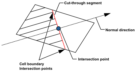
The concept of piecewise linear interface construction (PLIC) is also employed to construct the interface-front. The procedure for the interface–front reconstruction can be briefly described as follows and as shown in Figure 14.5: Schematic View of the Interface Cut Through the Front Cell:
Locate the interface front cells, where the sign(
 ) is alternating or the
value of the volume fraction is between 0 and 1, that is, a partially
filled cell.
) is alternating or the
value of the volume fraction is between 0 and 1, that is, a partially
filled cell.Calculate the normal of the interface segment in each front cell from the level-set function gradients.
Position the cut-through, making sure at least one corner of the cell is occupied by the designated phase in relation to the neighboring cells.
Find the intersection between the cell centerline normal to the interface and the interface so that the VOF is satisfied.
Find the intersection points between the interface line and the cell boundaries; these intersection points are designated as front points.
Once the interface front is reconstructed, the procedure for the minimization of the distance from a given point to the interface can begin as follows:
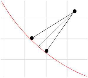
Calculate the distance of the given point in the domain to each cut-segment of the front cell. The method for the distance calculation is as follows:
If the normal line starting from the given point to the interface intersects within the cut-segment, then the calculated distance will be taken as the distance to the interface.
If the intersection point is beyond the end points of the cut-segment, the shortest distance from the given point to the end points of the cut-segment will be taken as the distance to the interface cut-segment, as shown in Figure 14.6: Distance to the Interface Segment.
Minimize all possible distances from the given point to all front cut-segments, so as to represent the distance from the given point to the interface. Thus, the values of these distances will be used to re-initialize the level-set function.
The current implementation of the model is only suitable for two-phase flow regime, where two fluids are not interpenetrating.
The level-set model can only be used when the VOF model is enabled.
The following features are not supported with the coupled VOF Level Set model:
Mass transfer
Periodic boundaries
Polyhedral meshes
Dynamic meshes
Overset meshes