


You can use Fluent to model interphase species mass transfer. Interphase species mass transfer can occur across a phase interface (between a gas and a liquid, or between a liquid and a solid) depending directly on the concentration gradient of the transporting species in the phases. For example,
evaporation of a liquid into a gaseous mixture including its vapor, such as the evaporation of liquid water into a mixture of air and water vapor.
absorption/dissolution of a dissolved gas in a liquid from a gaseous mixture. For example, the absorption of oxygen by water from air.
The interphase species mass transfer can be solved in either the Mixture model or the Eulerian model subject to the following conditions:
Both phases consist of mixtures with at least two species, and at least one of the species is present in both phases.
The two mixture phases are in contact and separated by an interface.
Species mass transfer can only occur between the same species from one phase to the other. For example, evaporation/condensation between water liquid and water vapor.
As in all interphase mass transfer models in Fluent, if a gas mixture is involved in an interphase species mass transfer process, it is always treated as a “to”-phase and the liquid mixture as a “from”-phase.
For the species involved in the mass transfer, the mass fractions in both phases must be determined by solving transport equations. For example, the mass fractions of water liquid and water vapor in an evaporation/condensation case must be solved directly from the governing equations, rather than algebraically or from the physical constraint relations.
To model interphase species mass transfer, phase species transport
equations are solved along with the phase mass, momentum and energy
equations. The transport equation for  , the local mass fraction of species
  in phase
  , is:
, is:
 | (14–640) |
where  denotes the pth phase, and
  is the number of phases in the system.
  ,
,  , and
, and  are the phase volume fraction, density, and velocity for the qth phase.
  is the net rate of production of homogeneous species
  through chemical reaction in phase
  .
.  is the rate of production from external sources, and
  is the heterogeneous reaction rate.
  denotes the mass transfer source from species
  on phase
  to species
  on phase
  .
.
In practice, the source term for mass transfer of a species between phase  and phase
  is treated as a single term,
  , depending on the direction of the mass transfer. The volumetric rate of
species mass transfer is assumed to be a function of mass concentration gradient of the
transported species.
, depending on the direction of the mass transfer. The volumetric rate of
species mass transfer is assumed to be a function of mass concentration gradient of the
transported species.
 | (14–641) |
where  is the volumetric mass transfer coefficient between the
pth phase and the qth phase,
is the volumetric mass transfer coefficient between the
pth phase and the qth phase,
 is the interfacial area, and
  is the mass concentration of species
  in phase
  , and
, and  is the mass concentration of species
  in phase . The derivation of the formulation of the volumetric rate of species mass
transfer is presented in Modeling Approach.
in phase . The derivation of the formulation of the volumetric rate of species mass
transfer is presented in Modeling Approach.
In order to solve the species mass transfer it is necessary to determine appropriate values for  and
and  .
.
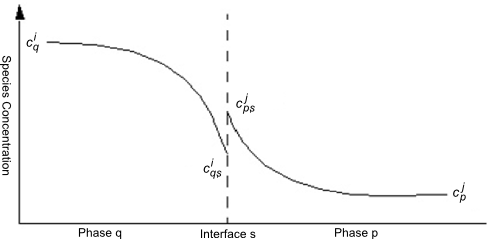
Interphase species mass transfer is modeled using the two-resistance model in Ansys Fluent. In situations where there are discontinuities in phase concentrations at dynamic equilibrium, it is in general not possible to simulate multi-component species mass transfer with the use of a single overall mass transfer coefficient. The two-resistance model, first proposed by Whitman [707], is a general approach analogous to the two-resistance heat transfer models. It considers separate mass transfer processes with different mass transfer coefficients on either side of the phase interface.
Consider a single species dissolved in the qth and pth phases with concentration of  and
and  , respectively, and with a phase interface,
  . Interphase mass transfer from the qth phase to the pth phase involves three steps:
The transfer of species
 from the bulk qth phase to the phase interface,
  .
.The transfer of species
 across the phase interface. It is identified as species
  in the pth phase.
The transfer of species
 from the interface,
  , to the bulk pth phase.
The two-resistance model has two principal assumptions:
The rate of species transport between the phases is controlled by the rates of diffusion through the phases on each side of the interface.
The species transport across the interface is instantaneous (zero-resistance) and therefore equilibrium conditions prevail at the phase interface at all times.
In other words, there exist two “resistances” for species transport between two phases, and they are the diffusions of the species from the two bulk phases  and
and  to the phase interface,
  . This situation is illustrated graphically in Figure 14.15: Distribution of Molar Concentration in the Two-Resistance Model.
Using Equation 14–641 with the assumption that  and
and  are the mass transfer coefficients for the qth and pth phases, respectively, the volumetric rates of phase mass exchange can be expressed as follows:
From the interface to the qth phase,
 | (14–642) |
From the interface to the pth phase,
 | (14–643) |
Under the dynamic equilibrium condition on the phase interface the overall mass balance must be satisfied:
 | (14–644) |
At the interface, the equilibrium relation given in Equation 14–650 also applies:
 | (14–645) |
where  are the equilibrium ratios for mass concentration.
From Equation 14–642 — Equation 14–645, one can determine the interface mass concentrations:
 | (14–646) |
and then obtain the interface mass transfer rates:
 | (14–647) |

The phase-specific mass transfer coefficients,  and
and  , can each be determined from one of the methods described in Mass Transfer Coefficient Models. It is also possible to specify a zero-resistance condition on one side of the interface. This is equivalent to an infinite phase-specific mass transfer coefficient. For example, if
  its effect is to force the interface concentration to be the same as the bulk concentration in phase
  . In addition, if the overall mass transfer coefficient is known,
  can be specified directly by a constant or a user-defined function.
Equilibrium models are used to compute equilibrium ratios  in Equation 14–641. The equilibrium models consider the case in which the species on the two phases are in dynamic equilibrium. The interphase mass transfer rate is determined from the relationship between the equilibrium species concentrations on the two phases.
Typically at equilibrium the species concentrations on the two phases are not the same. However, there exists a well-defined equilibrium curve relating the two concentrations. For binary mixtures, the equilibrium curve depends on the temperature and pressure. For multi-component mixtures, it is also a function of the mixture composition. The equilibrium curve is usually monotonic and nonlinear, and is often expressed in terms of equilibrium mole fractions of species  and
and  on phases
  and
and  :
:
 | (14–648) |
The simplest curve or relationship is quasi-linear and assumes that at equilibrium the mole fractions of the species between the phases are in proportion:
 | (14–649) |
where  is the mole fraction equilibrium ratio. This relationship can, alternatively, be expressed in terms of
  ,
,  , or
, or  :
:
 | (14–650) |
where  ,
,  , and
, and  are the equilibrium ratios for molar concentration, mass concentration, and mass fraction, respectively. These equilibrium ratios are related by the following expression:
 | (14–651) |
There are several well-known interphase equilibrium models to define or determine  for various physical processes. Ansys Fluent offers three ways to determine
  :
:
To quantify the concentration of a species,  , in phase
  , several different, but related, variables are used:
|
| |
|
| |
|
| |
|
|


These four quantities are related as follows:

where  is the sum of the molar concentrations of all species in phase
  , and
, and  is the phase density of phase
  .
.
In gas-liquid systems, the equilibrium relations are most conveniently expressed in terms of the partial pressure of the species in the gas phase. It is well known that for a pure liquid in contact with a gas mixture containing its vapor dynamic equilibrium occurs when the partial pressure of the vapor species is equal to its saturation pressure (a function of temperature). Raoult’s law extends this statement to an ideal liquid mixture in contact with a gas. It states that the partial pressure of the vapor species in phase  ,
,  , is equal to the product of its saturation pressure,
  , and the molar fraction in the liquid phase,
  :
:
 | (14–652) |
If the gas phase behaves as an ideal gas, then Dalton’s law of partial pressure gives:
 | (14–653) |
Using Equation 14–649, Equation 14–652, and Equation 14–653, Raoult’s law can be rewritten in terms of a molar fraction ratio:
 | (14–654) |
where the equilibrium ratio,  . While Raoult’s law represents the simplest form of the vapor-liquid equilibrium (VLE) equation, keep in mind that it is of limited use, as the assumptions made for its derivation are usually unrealistic. The most critical assumption is that the liquid phase is an ideal solution. This is not likely to be valid, unless the system is made up of species of similar molecular sizes and chemical nature, such as in the case of benzene and toluene, or n-heptane and n-hexane (see Vapor Liquid Equilibrium Theory).
Raoult’s Law applies only for a phase with an ideal liquid mixture. To handle the case of a gas species dissolved into a non-ideal liquid phase, Henry’s law provides a more generalized equilibrium relationship by replacing the saturation pressure,  , in Equation 14–652 with a constant,
  , for the liquid species
  , referred to as Henry’s constant:
 | (14–655) |
 has units of pressure and is known empirically for a wide range of materials, in particular for common gases dissolved in water. It is usually strongly dependent on temperature. The above form of Henry’s laws is typically valid for a dilute mixture (mole fraction less than 0.1) and low pressures (less than 20 bar) [602].
As with Raoult’s law, Henry’s law can be combined with Dalton’s law to yield an expression in terms of equilibrium ratio:
 | (14–656) |
where the equilibrium ratio is  .
.
In addition to the molar fraction Henry’s constant,  , the molar concentration Henry’s constant,
  is also commonly used:
 | (14–657) |
Fluent offers three methods for determining the Henry’s constants: constant, the Van’t Hoff correlation, and user-defined. In the Van’t Hoff correlation, the Henry’s constant is a function of temperature:
 | (14–658) |
and
 | (14–659) |
where  is the enthalpy of solution and
  is the Henry’s constant at the reference temperature,
  . The temperature dependence is:
 | (14–660) |
When using the Van’t Hoff correlation in Fluent you specify the value of the reference Henry’s constant,  , and the temperature dependence defined in Equation 14–660. These are material-dependent constants and can be found in [569]. By default, the constants for oxygen are used. You can also choose user-defined constants.
Important: Regardless of the units selected in the Fluent user interface,  is always expressed in units of M/atm for consistency with the presentation in most reference data tables. Appropriate unit conversions are applied inside Fluent.
In situations where neither Raoult’s law nor Henry’s law apply, such as liquid-liquid extraction, or multiple species mass transfers, Fluent offers you the option to directly specify the equilibrium ratios. You may choose to specify the equilibrium ratio in the following forms:
Molar concentration equilibrium ratio, 
|
Molar fraction equilibrium ratio, 
|
Mass fraction equilibrium ratio, 
|
These specify the ratio of the concentration variable for the From-phase divided by that for the To-phase as defined in Equation 14–649 and Equation 14–650. You can specify either a constant value or a user-defined function.
In Fluent, the overall mass transfer coefficient ( in Equation 14–647) can be modeled as a
constant or a user-defined function (UDF). The phase mass transfer coefficient (for
instance, in Equation 14–647) is defined on either side
of the phase interface and can be modeled as a constant, a UDF, or a function of the
phase Sherwood number. In a phase , the Sherwood number
in Equation 14–647) can be modeled as a
constant or a user-defined function (UDF). The phase mass transfer coefficient (for
instance, in Equation 14–647) is defined on either side
of the phase interface and can be modeled as a constant, a UDF, or a function of the
phase Sherwood number. In a phase , the Sherwood number  is expressed as:
 | (14–661) |
where  is the diffusivity of the qth phase,
and
is the diffusivity of the qth phase,
and  is a characteristic length (such as a bubble or droplet diameter).
The mass transfer coefficient in phase ,  , is defined similarly to in Equation 14–661.
The Sherwood number is either specified as a constant or determined from one of several empirical correlations. These methods are detailed in the following sections:
When modeled as a constant, the constant volumetric mass transfer coefficient ( , , or ) is specified by the user.
In the Sherwood number method, the user specifies a constant value for  , and the phase mass transfer coefficient, , is computed from Equation 14–661.
The Ranz-Marshall model uses an analogous approach to that for the Ranz-Marshall heat transfer coefficient model. The expression for the Sherwood number for flow past a spherical particle has the same form as that for the Nusselt number in the context of heat transfer, with the Prandtl number replaced by the Schmidt number:
 | (14–662) |
where  is the Schmidt number of the qth phase
and
is the Schmidt number of the qth phase
and  is the relative
Reynolds number:
is the relative
Reynolds number:

where  and
and  are, respectively, the dynamic viscosity and density
of the qth phase.
are, respectively, the dynamic viscosity and density
of the qth phase.  is the magnitude of the relative velocity between
phases. The Ranz-Marshall model is based on boundary layer theory
for steady flow past a spherical particle. It generally applies under
the conditions:
is the magnitude of the relative velocity between
phases. The Ranz-Marshall model is based on boundary layer theory
for steady flow past a spherical particle. It generally applies under
the conditions:

Like the Ranz-Marshall model, the Hughmark model [262] for mass transfer coefficient is also analogous to its heat transfer coefficient counterpart. The Ranz-Marshall model is extended to a wider range of Reynolds numbers by the Hughmark correction:
 | (14–663) |
The Reynolds number crossover point is chosen to ensure continuity. The model should not be used outside of the recommended Schmidt number range.
The Higbie mass transfer coefficient model provides a mass transfer coefficient for interphase species mass transfer based on Higbie’s penetration theory [196]. The Higbie model uses the following correlation:
 | (14–664) |
where
 = liquid phase species diffusion coefficient = liquid phase species diffusion coefficient |
 , ,  , ,  = turbulent eddy dissipation, density, and viscosity of
the liquid phase, respectively = turbulent eddy dissipation, density, and viscosity of
the liquid phase, respectively |