


Harmonic response analyses are used to determine the steady-state response of a linear structure to loads that vary sinusoidally (harmonically) with time, therefore enabling you to verify whether or not your designs will successfully overcome resonance, fatigue, and other harmful effects of forced vibrations.
Introduction
In a structural system, any sustained cyclic load will produce a sustained cyclic or harmonic response. Harmonic analysis results are used to determine the steady-state response of a linear structure to loads that vary sinusoidally (harmonically) with time, therefore enabling you to verify whether or not your designs will successfully overcome resonance, fatigue, and other harmful effects of forced vibrations.
This analysis technique calculates only the steady-state, forced vibrations of a structure. The transient vibrations, which occur at the beginning of the excitation, are not accounted for in a harmonic analysis.
In this analysis all loads as well as the structure’s response vary sinusoidally at the same frequency. A typical harmonic analysis will calculate the response of the structure to cyclic loads over a frequency range (a sine sweep) and obtain a graph of some response quantity (usually displacements) versus frequency. "Peak" responses are then identified from graphs of response vs. frequency and stresses are then reviewed at those peak frequencies.
Points to Remember
A harmonic response analysis is a linear analysis. Some nonlinearities, such as plasticity will be ignored, even if they are defined. All loads and displacements vary sinusoidally at the same known frequency (although not necessarily in phase). If the Reference Temperature is set as and that temperature does not match the environment temperature, a thermally induced harmonic load will result (from the thermal strain assuming a nonzero thermal expansion coefficient). This thermal harmonic loading is ignored for all harmonic analysis.
Mechanical offers the following options for the Solution Method property:
- Mode Superposition (Default)
For the (also called "MSUP") option, the harmonic response to a given loading condition is obtained by performing the necessary linear combinations of the eigensolutions obtained from a Modal analysis.
For MSUP, it is advantageous for you to select an existing modal analysis directly (although Mechanical can automatically perform a modal analysis behind the scene) since calculating the eigenvectors is usually the most computationally expensive portion of the method. In this way, multiple harmonic analyses with different loading conditions could effectively reuse the eigenvectors. For more details, refer to Harmonic Response Analysis Using Linked Modal Analysis System.
Acceleration and/or Displacement applied as a base excitation uses the Enforced Motion Method. See the Enforced Motion Method for Mode Superposition Transient and Harmonic Analyses section of the Mechanical APDL Structural Analysis Guide for additional information.
- Full
Using the Full option, you obtain harmonic response through the direct solution of the simultaneous equations of motion. In addition, a Harmonic Response analysis can be linked to, and use the structural responses of, a Static-Structural analysis. See the Harmonic Analysis Using Pre-Stressed Structural System section of the Help for more information.
- Include Residual Vector
This property is available when the Solution Method is set to . You can turn the Include Residual Vector property to execute the RESVEC command and calculate residual vectors.
Note: The following boundary conditions do not support residual vector calculations:
Nodal Force
Remote Force scoped to a Remote Point (created via Model object)
Moment scoped to a Remote Point (created via Model object)
- Variational Technology
Using the option, the application evaluates the harmonic response for each excitation frequency based on one direct solution.
- Program Controlled
Using the option, the application selects the best solution method based on the model. Internally, the application chooses either the or solution method.
- Krylov
The solution method enables you to quickly perform an approximate solution. This method is more computationally efficient than the method if solved for a large number of frequency values. See the Frequency-Sweep Harmonic Analysis via the Krylov Method section of the Mechanical APDL Structural Analysis Guide for more information.
Note:
For more technical information about Variational Technology, see the Harmonic Analysis Variational Technology Method section of the Mechanical APDL Theory Reference.
Also see the HROPT command in the Mechanical APDL Command Reference for more information about harmonic analysis options.
If a Command (APDL) object is used with the MSUP method, object content is sent twice; one for the modal solution and another for the harmonic solution. For that reason, harmonic responses are double if a load command is defined in the object, for example, F command.
Preparing the Analysis
As needed throughout the analysis, refer to the Steps for Using the Application section for an overview the general analysis workflow.
Define Engineering Data
Both Young's modulus (or stiffness in some form) and density (or mass in some form) must be defined. Material properties must be linear but can be isotropic or orthotropic, and constant or temperature-dependent. Nonlinear properties, if any, are ignored.
Define Connections
Any nonlinear contact such as Frictional contact retains the initial status throughout the harmonic analysis. The stiffness contribution from the contact is based on the initial status and never changes.
The application accounts for spring stiffness as well as damping when using the , , , and solution methods. For the option, the application ignores damping from springs.
Establish Analysis Settings
For a Harmonic Response analysis, the basic Analysis Settings include:
- Step Controls
The Step Controls category enables you to define step controls for an analysis that includes multiple load steps. You use the properties of this category to define the load steps and their options. When you select the Analysis Settings object, the content of the Step Controls category automatically displays in the Worksheet. You can modify certain properties in either the Worksheet or in the Details pane. For each load step, you can specify solution settings (Frequency Spacing, minimum frequencies, maximum frequencies, etc.). See the Step Controls for Harmonic Analysis Types section for a description of the properties.
- Options
The Options category enables you to specify the frequency range and the number of solution points at which the harmonic analysis will be carried out as well as the solution method to use and the relevant controls.
The Solution Method property options for a harmonic response analysis, , , Direct Integration (), and , are described below.
: The application selects the best solution method based on the model. Internally, the application chooses either the or solution method.
Mode Superposition: This is the default method and generally provides results faster than the other methods. Using this method, a modal analysis is first performed to compute the natural frequencies and mode shapes. Then the mode superposition solution is carried out where these mode shapes are combined to arrive at a solution. The Mode Superposition method cannot be used if you need to apply imposed (nonzero) displacements. When using this method, you can set the Cluster Results property to to group the structure's natural frequencies. This results in a smoother, more accurate tracing of the response curve. The default method of equally spaced frequency points can result in missing the peak values. See the Options section for more information about the cluster property.
The method also includes the following additional properties:
- On Demand Expansion Option
Options for this property include (default), , and . When set to , an additional read-only property, On Demand Expansion, displays. This property only displays for the option and the application determines the value for the property, either or .
When the On Demand Expansion Option property is set to , either manually or from the setting, the application creates the result file optimally. The application evaluates the results using the Modal solution data and calculates any other results “on demand.” This improves solution performance and reduces file size. In addition, the application automatically removes mode shape data from the result file as determined by the On Demand Mode Shape preference.
You can change the default setting for the On Demand Expansion Option property and the On Demand Mode Shape preference using the Options (Modal, Harmonic and Transient Mode Superposition) category of the Analysis Settings and Solution group in the Options dialog.
- Store Results At All Frequencies
When you set the Store Results At All Frequencies property to No, the application requests that only minimal data be retained. Only the harmonic results requested at the time of solution are calculated. The availability of the results is therefore not determined by the settings in the Output Controls.
Note: With this option set to No, the addition of new frequency or phase responses to a solved environment requires a new solution. Adding a new contour result of any type (stress or strain) or a new probe result of any type (reaction force or reaction moment) for the first time on a solved environment requires you to solve, but adding additional contour results or probe results of the same type does not share this requirement; data from the closest available frequency is displayed (the reported frequency is noted on each result).
New and/or additional displacement contour results as well as bearing probe results do not share this requirement. These results types are basic data and are available by default.
The values of frequency, type of contour results (stress or strain) and type of probe results (reaction force, reaction moment, or bearing) at the moment of the solution determine the contents of the result file and the subsequent availability of data. Planning these choices can significantly reduce the need to re-solve an analysis.
Caution: Use caution when adding result objects to a solved analysis. Adding a new result invalidates the solution and requires the system to be re-solved, even if you were to add and then delete a result object.
Full: Calculates all displacements and stresses in a single pass. Its main disadvantages are:
It is more "expensive" in CPU time than the Mode Superposition method.
It does not allow clustered results, but rather requires the results to be evenly spaced within the specified frequency range.
: Instead of using the full matrices to compute the results, the application computes the solution at the middle of the requested frequency range and then interpolates the system matrices and loading on the entire frequency range to approximate the results across the range.
: For pure acoustic Coupled Field Harmonic, pure acoustic Harmonic Acoustics, and Harmonic Response analyses, use this option to reduce the entire system of equations and build a Krylov Subspace set of vectors at the middle of the frequency range. The application solves this reduced system and then expands the solution over the entire frequency range.
- Damping Controls
These properties enable you to specify damping for the structure in the Harmonic Response analysis. Controls include: Eqv. Damping Ratio From Modal (MSUP method), Damping Ratio (MSUP method), Constant Structural Damping Coefficient, Stiffness Coefficient (beta damping), and a Mass Coefficient (alpha damping). They can also be applied as Material Damping using the Engineering Data tab.
Note: You can apply element damping using Springs and Bearings. The damping from the elements is supported for a Harmonic Response analysis when the Solution Method property is set to and for a linked Mode Superposition Harmonic Response analysis when the Damped property (Analysis Settings > Solver Controls) in the upstream Modal analysis is set to . See the Damping section in the Structural Analysis Guide of Mechanical APDL documentation for more information.
Important: If multiple damping specifications are made the effect is cumulative.
- Analysis Data Management
These properties enable you to save solution files from the harmonic analysis. The default behavior is to only keep the files required for postprocessing. You can use these controls to keep all files created during solution or to create and save the Mechanical APDL application database (db file).
Define Initial Conditions
Currently, the initial conditions Initial Displacement and Initial Velocity are not supported for Harmonic analyses.
For a Pre-Stressed Full Harmonic analysis, the preloaded status of a structure is used as a starting point for the Harmonic analysis. That is, the static structural analysis serves as an Initial Condition for the Full Harmonic analysis. See the Applying Pre-Stress Effects section of the Help for more information.
Note:
In the Pre-Stressed MSUP Harmonic Analysis, the pre-stress effects are applied using a Modal analysis.
When you link your Harmonic (Full) analysis to a Structural analysis, all structural loading conditions, including Inertial loads, such as Acceleration and Rotational Velocity, are deleted from the Full Harmonic Analysis portion of the simulation once the loads are applied as initial conditions (via the Pre-Stress object). Refer to the Mechanical APDL command PERTURB,HARM,,,DZEROKEEP for more details.
If displacement loading is defined with Displacement, Remote Displacement, Nodal Displacement, or Bolt Pretension (specified as , , or ) loads in the Static Structural analysis, these loads become fixed boundary conditions for the Harmonic solution. This prevents the displacement loads from becoming a sinusoidal load during the Harmonic solution.
Apply Boundary Conditions
The Harmonic Response analysis supports the following boundary conditions:
- Inertial
Acceleration (Phase Angle is not supported.)
- Loads
Pipe Pressure (line bodies only) - Not supported for MSUP Solution Method.
Force (applied to a face, edge, or vertex)
Bearing Load (Phase Angle is not supported.)
Given a specified Displacement
- Supports
Any type of Support can be used in harmonic analyses.
Note: The Compression Only support is nonlinear but should not be utilized even though it behaves linearly in harmonic analyses.
- Conditions
- Direct FE (node-based Named Selection scoping and constant loading only)
Nodal Orientation (Phase Angle is not supported.)
- Base Excitation (MSUP Only)
Acceleration as a base excitation.
Displacement as a base excitation.
Important: When duplicating an analysis within Mechanical that includes loads with the Base Excitation property set to (Acceleration and/or Displacement), these loads will lose their scoping during the duplication process.
Note: Support for boundary conditions varies for a Harmonic Response analysis that is linked to either a Static-Structural or Modal analysis. See the Harmonic Response Analysis Using Linked Modal Analysis System or the Harmonic Analysis Using Pre-Stressed Structural System sections of the Help for specific boundary condition support information.
In a Harmonic Response Analysis, boundary condition application has the following requirements:
You can apply multiple boundary conditions to the same face.
All boundary conditions must be sinusoidally time-varying.
Transient effects are not calculated.
All boundary conditions must have the same frequency.
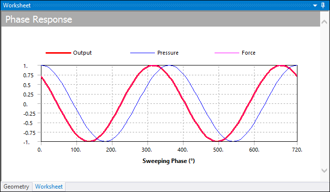
Boundary conditions supported with the Phase Angle property allow you to specify a phase shift that defines how the loads can be out of phase with one another. As illustrated in the example Phase Response below, the pressure and force are 45o out of phase. You can specify the preferred unit for phase angle (in fact all angular inputs) to be degrees or radians using the Units option in the Tools group of the Home tab.
An example of a Bearing Load acting on a cylinder is illustrated below. The Bearing Load, acts on one side of the cylinder. In a harmonic analysis, the expected behavior is that the other side of the cylinder is loaded in reverse; however, that is not the case. The applied load simply reverses sign (becomes tension). As a result, Ansys recommends avoid the use of Bearing Loads in this analysis type.
Solve
Solution Information continuously updates any listing output from the solver and provides valuable information on the behavior of the structure during the analysis.
Review Results
Result specification for Harmonic Response analyses includes:
- Contour Plots
Contour plots include stress, elastic strain, and deformation, and are basically the same as those for other analyses. If you wish to see the variation of contours over time for these results, you must specify an excitation frequency and a phase. The Sweeping Phase property in the details view for the result is the specified phase, in time domain, and it is equivalent to the product of the excitation frequency and time. Because Frequency is already specified in the Details view, the Sweeping Phase variation produces the contour results variation over time. The Sweeping Phase property defines the parameter used for animating the results over time. You can then see the total response of the structure at a given point in time, as shown below.
Setting the Amplitude property to enables you to see the amplitude contour plots at a specified frequency. Additionally, a read-only Coordinate System property displays when this property is set to , and is automatically set to , the only supported coordinate system. For additional information about Amplitude calculation for derived results, see the next section, Amplitude Calculation in Harmonic Analysis.
Since each node may have different phase angles from one another, the complex response can also be animated to see the time-dependent motion.
- Frequency Response and Phase Response
Frequency Response and Phase Response charts which give data at a particular location over an excitation frequency range and a phase period (the duration of the Phase Response results, respectively). Graphs can be either Frequency Response graphs that display how the response varies with frequency or Phase Response plots that show how much a response lags behind the applied loads over a phase period.
Note: You can create a contour result from a Frequency Response result type in a Harmonic Analysis using the Create Contour Result feature. This feature creates a new result object in the tree with the same Type, Orientation, and Frequency as the Frequency Response result type. However, the Phase Angle of the contour result has the same magnitude as the frequency result type but an opposite sign (negative or positive). The sign of the phase angle in the contour result is reversed so that the response amplitude of the frequency response plot for that frequency and phase angle matches with the contour results.
- Fatigue Tool
You can use the Fatigue Tool to view fatigue results for the repeated loading of a particular Frequency and Phase Angle.
- Waterfall Diagrams/Mode Contribution
If your analysis contains multiple RPM steps, you can use Waterfall Diagram results and the Mode Contribution result. These result types are useful when analyzing the Noise Vibration Harshness (NVH) footprint of a device for the frequencies of all RPMs.