


This feature allows you to relate the motion of different portions of a model through the use of an equation. The equation relates the degrees of freedom (DOF) of one or more Remote Points for Coupled Field Analyses, Harmonic Response, Harmonic Acoustics, Modal, Modal (Samcef), Static Structural, Static Structural (Samcef), or Transient Structural systems, or one or more joints for the Ansys Rigid Dynamics solver.
For example, the motion along the X direction of one remote point (Remote Point A) could be made to follow the motion of another remote point (Remote Point B) along the Z direction by:
0 = [1/mm ∙ Remote Point A (X Displacement)] - [1/mm ∙ Remote Point B (Z Displacement)]
The equation is a linear combination of the DOF values. Thus, each term in the equation is defined by a coefficient followed by a node (Remote Point) and a degree of freedom label. Summation of the linear combination may be set to a non-zero value. For example:
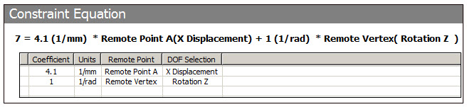
7 = [4.1/mm ∙ Remote Point A (X Displacement)] + [1/rad ∙ Remote Vertex (Rotation Z)]
Similarly, for the Ansys Rigid Dynamics solver, to make the rotational velocity of gear A (Revolute A) to follow the rotational velocity of gear B (Revolute B), in the Z direction, the following constraint equation should be written:
0 = [1/rad ∙ Revolute A (Omega Z)] - [1/rad ∙ Revolute B (Omega Z)]
This equation is a linear combination of the Joints DOF values. Thus, each term in the equation is defined by a coefficient followed by a joint and a degree of freedom label. Summation of the linear combination may be set to a non-zero value. For example:
7 = [4.1/mm ∙ Joint A (X Velocity)] + [1/rad ∙ Joint B (Omega Z)]
Note that the Joints DOF can be expressed in terms of velocities or accelerations. However, all terms in the equation will be based on the same nature of degrees of freedom, that is, all velocities or all accelerations.
To apply a constraint equation support:
Insert a Constraint Equation object by:
Selecting from the Conditions drop-down menu on the Context tab.
Or...
Right-clicking on the environment object and selecting .
In the Details pane, enter a constant value that will represent one side of the constraint equation. The default constant value is zero.
In the Worksheet, right-click in the first row and choose Add, then enter data to represent the opposite side of the equation. For the first term of the equation, enter a value for the Coefficient, then select entries for Remote Point or Joint and DOF Selection. Add a row and enter similar data for each subsequent term of the equation. The resulting equation displays as you enter the data.
Using the example presented above, a constant value of 7 is entered into the Details pane, and the data shown in the table is entered in the Worksheet.
Note: For Harmonic, Modal, Static Structural, and Transient Structural systems, the first unique degree of freedom in the equation is eliminated in terms of all other degrees of freedom in the equation. A unique degree of freedom is one which is not specified in any other constraint equation, coupled node set, specified displacement set, or master degree of freedom set. You should make the first term of the equation be the degree of freedom to be eliminated. Although you may, in theory, specify the same degree of freedom in more than one equation, you must be careful to avoid over-specification.
Constraint Equation Characteristics
In the Worksheet, you can insert rows, modify an existing row, or delete a row.
A local coordinate system is defined in each remote point that is used.
The constant term is treated as a value with no unit of measure.
Coefficients for X Displacement, Y Displacement, Z Displacement, X Velocity, Y Velocity, Z Velocity, X Acceleration, Y Acceleration, and Z Acceleration have a unit of 1/length.
Coefficients for Rotation X, Rotation Y, Rotation Z, Omega X, Omega Y, Omega Z, Omega Dot X, Omega Dot Y, and Omega Dot Z have a unit of 1/angle. Note that in a velocity-based constraint equation, coefficients use angle units and not rotational velocity units.
If you change a DOF such that the unit type of a coefficient also changes (for example, rotation to displacement, or vice versa), then the coefficient resets to 0.
You can parameterize the constant value entered in the Details pane.
The state for the Constraint Equation object will be under-defined (? in the tree) under the following circumstances:
There are no rows with valid selections.
Remote Points being used are underdefined or suppressed.
Joints being used are underdefined or suppressed.
The analysis type does not support this feature.
The selected DOFs are invalid for the analysis (2D versus 3D, or remote point versus joints DOFs).
The graphic user interface does not check for overconstraint.
API Reference
For specific scripting information, see the Constraint Equation section of the ACT API Reference Guide.