


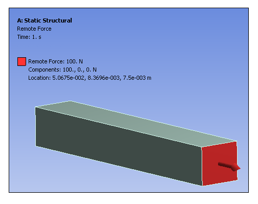
A Remote Force is equivalent to a regular force load on a face or a force load on an edge, plus some moment. A Remote Force can be applied to a face, edge, vertex, element face, or node of a 3D model, or to an edge, vertex, or node of a 2D model.
A Remote Force can be used as an alternative to building a rigid part and applying a force load to it. The advantage of using a Remote Force load is that you can directly specify the location in space from which the force originates.
A Remote Force is classified as a remote boundary condition. Refer to the Remote Boundary Conditions section for a listing of all remote boundary conditions and their characteristics.
This page includes the following sections:
| Analysis Types |
| Dimensional Types |
| Geometry Types |
| Topology Selection Options |
| Define By Options |
| Magnitude Options |
| Applying a Remote Force Boundary Condition |
| Details Properties |
| API Reference |
Analysis Types
Remote Force is available for the following analysis types:
Dimensional Types
The supported dimensional types for the Remote Force boundary condition include:
3D Simulation
2D Simulation: Not supported for Explicit Dynamics.
Geometry Types
The supported geometry types for Remote Force include:
Solid
Surface/Shell
Wire Body/Line Body/Beam
Topology Selection Options
The supported topology selection options for the Remote Force boundary condition include:
Face: Supported for 3D only.
Edge
Vertex
Cannot be applied to a vertex scoped to an end release.
Vertex selections do not support the Behavior option.
Node
Element Face: Supported for 3D only.
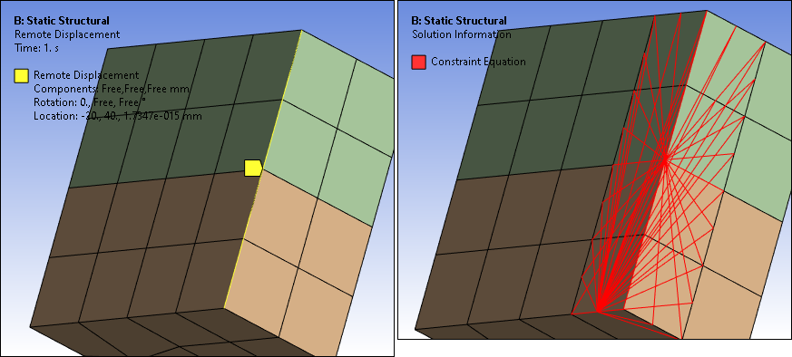
- Applying Remote Loads to a Straight Edge
If you apply a remote load to a straight edge (with colinear nodes) of a deformable surface body or a solid body, the application applies the load to the edge as well as the neighboring nodes of the element faces of the deformable surface body or the solid body, respectively. This transfers the rotations of the pilot node (of the Remote Point) to the surface or solid body.
Exception: If you scope a remote load to a deformable beam, the application internally changes the setting of the Behavior property to and prompts you with a warning.
The following example shows how the application applies a Remote Displacement, scoped to a straight edge, to the neighboring element face nodes. In this example, the imbalance of constraint equations created on the blocks might result in unwanted non-zero moment reactions. You can minimize this by using either a lower order mesh or a coarser higher order mesh. For more information, see the Surface-Based Constraints section of the Mechanical APDL Contact Technology Guide.
Define By Options
The supported Define By options for the Remote Force boundary condition include:
. While loads are associative with geometry changes, load directions are not. This applies to any load that requires a vector input.
The vector load definition displays in the Annotation legend with the label Components. The Magnitude and Direction entries, in any combination or sequence, define these displayed values. These are the values sent to the solver.
: Supported for Harmonic Response analysis only.
: Supported for Harmonic Response analysis only.
Magnitude Options
The Magnitude options for Remote Force include:
Constant
Tabular (Time Varying)
Tabular (Step Varying): Supported for Static Structural analysis only.
Tabular (Frequency Varying): Supported for Harmonic Response Analysis only. By default, at least two frequency entries are required when defining a frequency dependent tabular load.
Tabular (Harmonic Index Varying): Supported for Harmonic Response (Full) analysis only when Cyclic Region is defined. By default, at least two harmonic index entries are required when defining a Harmonic Index dependent tabular load.
Tabular (Sector Number): Supported for Harmonic Response (Full) analysis only when a Cyclic Region is defined. By default, at least two entries are required to define a dependent tabular load.
Function (Time Varying)
Applying a Remote Force Boundary Condition
You apply a Remote Force as you would apply a force load except that the location of the load origin can be replaced anywhere in space either by picking or by entering the XYZ locations directly or by scoping a geometric entity using the Location property. Note that when you first define the properties of the Remote Force, the application automatically sets the default location of the Location property at the centroid of the scoped geometry selection(s). This setting is maintained even if you re-specify your geometry scoping. It is necessary to manually change the Location property's definition.
The location and the direction of a Remote Force can be defined in the Global Coordinate System or in a local coordinate system.
To apply a Remote Force:
On the Environment Context tab, open the Loads drop-down menu and select . Alternatively, right-click the Environment tree object or in the Geometry window and select Insert>.
Define the Scoping Method as either Geometry Selection, Named Selection, or Remote Point and then specify the scoping.
Tip: For a project where none of the analyses have been solved, automatic Remote Point creation (promotion) is available in Harmonic Response or Transient Structural analyses that use a linked Modal system to implement the Mode Superposition (MSUP) solver method. To use this feature:
Select a supported topology (geometric or mesh entity) on your model, and
Insert a Remote Force load.
The application automatically creates a corresponding Remote Point for the specified load and scopes the load to that Remote Point. Automatic Remote Point creation improves processing performance by eliminating the need to create internal elements for the load.
Specify a coordinate system as needed. The default selection is the Global Coordinate System. You can also specify a user-defined or local coordinate system.
Select the method used to define the Remote Force: (default), , , or .
Define the Magnitude, Coordinate System directional loading, and/or Direction of the load based on the above selections.
Note:If you scope this load using the Element Face or Node selection options, you must use either of these options to properly specify the Direction property. That is, select the Direction property field (Click to Define), make sure that either the Element Face or the Node selection option is active, and then define the desired direction.
The Direction property is not associative and does not remain joined to the entity(s) selected for its specification. Therefore, this direction is not affected by geometry updates, part transformation, or the Configure tool (for joints).
For Harmonic analyses, specify a Phase Angle as needed.
Select the Behavior of the geometry.
As needed, enter a Pinball Region value. The default value is .
If you are performing a Harmonic MSUP analysis that is linked to upstream system, you can set the Loading Application property to either (default) or . This property selection enables you to specify between applying the load using load vectors or tables in the harmonic analysis. The option is not available if you scope the load to a Remote Point or a vertex.
Note: Since it is considered a remote boundary condition, a Remote Force can make use of remote points that were either specifically defined or created internally by the application. To do a visual check, you can display the connection lines between your scoping and the remote point by selecting the Remote Point Connections option of the Style group (Display tab).
Details Properties
The selections available in the Details pane are described below.
| Category | Property/Options/Description | ||
|---|---|---|---|
| Scope |
Scoping Method: Options include:
Coordinate System: Drop-down list of available coordinate systems. is the default. The following properties are used to define the location of the load’s origin:
Location: This property specifies the location of the load's origin. The default location is the centroid of your geometry selection(s). You can define this property manually using geometry entity selections as well as by making entries in the above coordinate properties. | ||
| Definition |
Type: Read-only field that displays boundary condition type - Remote Force. Define By, options include:
Note: If you scope this load using the Element Face or Node selection options, you must use either of these options to properly specify the Direction property. That is, select the Direction property field (Click to Define), make sure that either the Element Face or the Node selection option is active, and then define the desired direction.
Note: Selection of a Coordinate System rotated out of the global Cartesian X-Y plane is not supported in a 2D analysis.
Suppressed: Include ( - default) or exclude () the boundary condition. Non-Cyclic Loading Type: This property is available for Full Harmonic Analysis when Cyclic Symmetry is present in the model. Options include:
Important: When you specify the load as Tabular, the Independent Variable property displays and is set to by default. The Harmonic Index property is hidden as their values are entered in the table.
Harmonic Index: This property displays when the Non-Cyclic Loading Type property is set to Harmonic Index. Where NS is Number of Sectors, enter a value from:
: This property displays when the Non-Cyclic Loading Type property is set to . You use this property to specify the desired sector onto which you want to apply the non-cyclic load. If you choose Tabular for the Magnitude property, you can then set the Independent Variable property to and then specify your loading using the Tabular Data window. Behavior: This option dictates the behavior of the attached geometry. If the Scope Method property is set to , the boundary condition will then assume the Behavior defined in the referenced Remote Point as well as other related properties. Options include:
Material: This property is available when the Behavior property is set to . Select a material to define material properties for the beams used in the connection. Density is excluded from the material definition. Radius: This property is available when the Behavior property is set to . Specify a radius to define the cross section dimension of the circular beam used for the connection. Follower Load (Rigid Dynamics analysis only): When set to (default), the force direction doesn't change during the simulation. When set to , the force direction is updated with the underlying body. | ||
|
Step Controls (Visible for Harmonic Response analysis with multiple load steps defined) |
Step Varying: Options include (default) and . When you select , the Remote Load is applicable at all defined steps. When set to , only the load step selected in either the RPM Selection or Step Selection properties described below is applicable. RPM Selection: This property displays when the Multiple Step Type property is set to . Specify a Step Selection value from the values available in the RPM Value property of the Analysis Settings object to use for the Remote Load. Step Selection: This property displays when the Multiple Step Type property of the Analysis Settings object is set to . Specify a Step Selection value from the values available in the Load Step Value property of the Analysis Settings object to use for the Remote Load. | ||
| Advanced |
Pinball Region: Modify the Pinball setting to reduce the number of elements included in the solver. Note: The Pinball Region property is not supported for the Samcef and ABAQUS solvers.
Loading Application (linked MSUP Harmonic analysis only): Options include (default) and . Using the option, the scale factor specified through load magnitude is applied to the load vector in MSUP Harmonic analysis. Using the option, the load magnitude is specified in tabular data format and is directly applied to the selected scoping in the MSUP Harmonic analysis. Note: The option is not available if you scope the load to a Remote Point or a vertex.
|
API Reference
For specific scripting information, see the Remote Force section of the ACT API Reference Guide.