The global Acceleration boundary condition defines a linear acceleration of a structure in each of the global Cartesian axis directions.
If desired, Acceleration can be used to simulate gravity (by using inertial effects) by accelerating a structure in the direction opposite of gravity (the natural phenomenon of). That is, accelerating a structure vertically upwards (+Y) at 9.80665 m/s2 (in metric units), applies a force on the structure in the opposite direction (-Y) inducing gravity (pushing the structure back towards earth). Units are length/time2.
Alternatively, you can use the Standard Earth Gravity load to produce the effect of gravity. Gravity and Acceleration are essentially the same type of load except they have opposite sign conventions and gravity has a fixed magnitude. For applied gravity, a body tends to move in the direction of gravity and for applied acceleration, a body tends to move in the direction opposite of the acceleration.
Acceleration as a Base Excitation
Acceleration can also be defined as a base excitation during a Mode Superposition Transient analysis or a Mode Superposition Harmonic Response analyses. You scope base excitations to a boundary condition. You can scope multiple base excitations to the same boundary condition, but the base excitations cannot have same direction specified (via the Direction property).
Important: When duplicating an analysis within Mechanical that includes loads with the Base Excitation property set to (Acceleration and/or Displacement), these loads will lose their scoping during the duplication process.
This page includes the following sections:
Analysis Types
Acceleration is available for the following analysis types:
Dimensional Types
Acceleration applies a uniform load over all bodies. The supported dimensional types include:
3D Simulation
2D Simulation
Geometry Types and Topology Selection Options
By virtue of Acceleration's physical characteristics, this boundary condition is always applied to all bodies of a model.
Define By Options
The supported Define By options for the Acceleration boundary condition include:
While loads are associative with geometry changes, load directions are not. This applies to any load that requires a vector input, such as Acceleration.
The vector load definition displays in the Annotation legend with the label Components. The Magnitude and Direction entries, in any combination or sequence, define these displayed values. These are the values sent to the solver.
: Supported for Acceleration as a Base Excitation for Harmonic Response analysis only.
: Supported for Acceleration as a Base Excitation for Harmonic Response analysis only.
Magnitude Options
The supported Magnitude options for Acceleration include the following:
Constant
Tabular (Time Varying)
Tabular (Step Varying): Supported for Static Structural and Rigid Dynamics analyses only.
Tabular (Frequency Varying): Supported for Harmonic Response analysis only. By default, at least two frequency entries are required when defining a frequency dependent tabular load.
Function (Time Varying): Not supported for Explicit Dynamics or LS-DYNA analyses.
For a Rigid Dynamics analysis, if the Acceleration is defined using an expression, you cannot also have a Standard Earth Gravity object.
Applying an Acceleration Boundary Condition
To apply an Acceleration:
On the Environment Context tab, click Inertial>Acceleration. Alternatively, right-click the Environment object in the tree or in the Geometry window and select Insert>Acceleration.
Select the method used to define the Acceleration: Options include (default) or .
Define the loading inputs: Magnitude, Coordinate System, and/or Direction of the Acceleration based on the above selections.
To apply Acceleration as a base excitation when the Solver Type property is defined as during a Transient (default setting for a Transient configured to a Modal solution) or a Mode-Superposition Harmonic Response analysis:
Set the Base Excitation property to .
The Boundary Condition property provides a drop-down list of the boundary conditions that correspond to the Acceleration. Make a selection from this list. Valid boundary conditions for excitations include:
Fixed Support
All Fixed Supports
Displacement
Remote Displacement
Nodal Displacement
Spring: Body-to-Ground
The Absolute Result property is set to by default. Change the value to if you do not want to include enforced motion.
Note: If you apply more than one base excitation (either Displacement or Acceleration), the Absolute Result property needs to have the same setting, either or .
As needed, set the Define By property to from (default).
For Harmonic analyses, specify a Phase Angle as needed.
Note: You can scope Acceleration or Displacement as a base excitation to the same boundary condition, but the base excitations cannot have the same direction specified (via the Direction property).
Details Pane Properties
The selections available in the Details pane are described below.
| Category | Property/Options/Description |
|---|---|
| Scope | Geometry: Read-only field indicating All
Bodies. Boundary Condition (Acceleration as a Base Excitation only): Drop-down list of available boundary conditions for application. |
| Definition |
Base Excitation (Acceleration as a Base Excitation only): is the default setting. Set to to specify the Acceleration as a Base Excitation. Absolute Result (Acceleration as a Base Excitation only): This option allows you to include enforced motion with ( - default) or without () base motion. Define By: Options for this property include the following:
Suppressed: Include () or exclude () the boundary condition. |
|
Step Controls (Visible for Harmonic Response analysis with multiple load steps defined) |
Step Varying: Options include (default) and . When you select , the Remote Load is applicable at all defined steps. When set to , only the load step selected in either the RPM Selection or Step Selection properties described below is applicable. RPM Selection: This property displays when the Multiple Step Type property is set to . Specify a Step Selection value from the values available in the RPM Value property of the Analysis Settings object to use for the Remote Load. Step Selection: This property displays when the Multiple Step Type property of the Analysis Settings object is set to . Specify a Step Selection value from the values available in the Load Step Value property of the Analysis Settings object to use for the Remote Load. Note: Step varying displacements can only be applied in one direction for all load steps, for a selected set of nodes. |
|
Load Vector Controls (Substructure Generation analysis only) |
Load Vector Assignment: Options include (default) and . When set to , the Load Vector Number property displays. Load Vector Number: Specify a Load Vector
Number using any value greater than |
Mechanical APDL References and Notes
The following Mechanical APDL commands and considerations are applicable for Acceleration:
Acceleration is applied using the ACEL command.
Magnitude (constant, tabular, and function) is always represented as a table in the input file.
Note:
Should both an Acceleration and a Standard Earth Gravity boundary condition be specified, a composite vector addition of the two is delivered to the solver.
In a Mode-Superposition Transient analysis, Standard Earth Gravity is not allowed in conjunction with Acceleration.
Condensed Parts
Important: When working with substructures, if the inertial acceleration is scoped to a Condensed Part, the nodes of the condensed part are not marked as the master degree of freedom. Instead, multiple super element load vectors are generated for each acceleration component via the substructure restart mechanism and scaled using SFE ,,SELV command. See the ANTYPE ,SUBSTR,RESTART command in the Mechanical APDL Command Reference. For additional information, see The CMS Generation Pass in the Substructuring Analysis Guide.
Limitation: If your analysis includes a Condensed Part, the application does not support Acceleration when the Step Varying property is set to .
Base Excitation
The following Mechanical APDL commands and considerations are applicable when Acceleration is defined as a base excitation in a Mode Superposition Transient analysis or a Mode Superposition Harmonic Response analysis:
Magnitude (constant or tabular) is always represented as a table in the input file.
Base excitation is defined using the D command under the Modal restart analysis (under Modal analysis in case of Standalone Harmonic Response analysis).
Base excitation is applied using the DVAL command during a Mode Superposition Transient analysis or Mode Superposition Harmonic Response analysis.
Note: Acceleration can be defined as base excitation in a Modal linked Harmonic Response and Modal linked Transient analysis only when the upstream Modal analysis Solver Type is set to (provided program sets solver type internally to , , or ).
API Reference
For specific scripting information, see the Acceleration section of the ACT API Reference Guide.
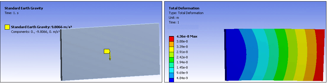
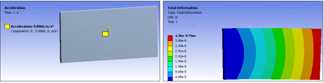
Acceleration and Standard Earth Gravity Examples
The following illustrations compare how Acceleration and Gravity can be used to specify a gravitational load with the same result:
Global Acceleration Load Applied in the +Y Direction to Simulate Gravity and Deformation Result
Standard Earth Gravity Applied and Deformation Result