


The Krylov Method is a fast approximate alternative for harmonic analyses and is meant for speed, rather than accuracy.
There are two methods to implement a harmonic analysis using the Krylov Method:
If you wish to customize your analysis, you can use the three macros described in Krylov Method Implemented via Macros as a modifiable template.
If you do not require customization, you can use the simpler procedure described in Krylov Method Implemented using Mechanical APDL Commands. Since implementation via Mechanical APDL commands runs an analysis identical to that defined by the three macros without any modifications, details of the analysis can be inferred directly from the macros. Additional details on the theory and equations describing the Krylov method can be found in the works of Puri [1] and Eser [2].
The performance improvement of the Krylov method comes with a potential tradeoff
on the accuracy of the final harmonic solution. To increase solution accuracy over a
wide frequency range, you can extend the single range procedure described here (see
also the Frequency-Sweep Analysis via the Krylov Method
in the overview section) by applying the Krylov method to analyze multiple
load steps, for example, multiple frequency ranges. For each frequency range, set
the frequency at which the subspace is built
(HROPT,KRYLOV,FRQKRY) closer to the
frequency of interest in that range. In general, the solution is more accurate in
the frequency range nearer to the frequency at which the subspace is built.
Additionally, the use of frequency-dependent matrices and/or loading may also affect
the accuracy because the subspace is built at a single frequency. The L2-norm of
calculated residuals across frequency range gives a good estimation of the error in
the harmonic response distribution, which can provide information on how to best
split the whole range into multiple ranges. Increasing subspace size
(MAXDIM on KRYOPT) can also improve
solution accuracy, especially for the high-frequency end of the range. Since there
is a computational cost and additional memory requirements associated with both
rebuilding the subspace and increasing the subspace size, you need to consider the
trade-off between improving accuracy and the associated efficiency loss.
Consider these additional distinctions, limitations, and tips when defining a harmonic analysis using the Krylov Method:
The procedures for building the model, applying loads, and reviewing the results are similar to those described for the full harmonic analysis except the loading, material properties, and real constants should be mostly frequency-independent (see Full Harmonic Analysis in the Structural Analysis Guide). While frequency-dependent matrices and loading can be included in the analysis, they impact the accuracy of the Krylov method.
Only supports single-field structural or acoustic anayses (coupled-field analyses are not supported)
Does not support unsymmetric matrices.
Linear Perturbation Analysis is supported.
Shared-memory parallel (SMP), distributed-memory parallel (DMP), and hybrid parallel are supported for the Krylov method implemented via Mechanical APDL commands. Only SMP is supported using the macros.
Frequency-based domain decomposition (DDOPTION,FREQ) in a DMP solution is supported.
User-defined frequencies (
FREQARRon HARFRQ) are supported. Details are similar to those discussed in dynamic options for a full harmonic analysis (see Forcing Frequency Range).Limitations for acoustics analyses:
The Helmholtz governing equation is used to model a pressure wave. The convective wave equation is not supported, and the mean flow effect is not taken into account.
The floquet periodic boundary condition (FPBC) and analytic incident wave source (AWAVE) for the acoustic excitation are not supported.
Acoustic fluid-structure interaction (FSI) is not supported.
Limitations for single-field structural analyses:
Cyclic symmetry and multistage cyclic symmetry analyses are not supported.
Lagrange multiplier based elements (joints/contact and mixed u-P) are not supported.
The solution commands used to specify a harmonic analysis using the Krylov method are listed in the table below.
Table 4.5: Solution Commands for a Krylov Method Harmonic Analysis
| Command | Description |
| /SOLU | Enter the solution processor |
| ANTYPE,HARMIC | Specify a harmonic analysis |
| HROPT,KRYLOV | Specify the Krylov solution method |
| KRYOPT | Optional command to specify nondefault solution options. |
| HARFRQ | Specify the forcing frequency range |
| NSUBST | Set the number of harmonic solutions |
| KBC | Specify ramped or step loading |
| SOLVE | Run the solution |
| FINISH | Exit the solution processor |
Example 4.1: Krylov Harmonic Analysis of a 1-D Wave in an Acoustic Duct
This example problem demonstrates the use of the frequency-sweep Krylov method to simulate a cylindrical acoustic duct with a 1-D wave with pressure excitation on one end and an impedance boundary condition on the opposite end. Results are compared to those obtained in a full harmonic analysis. The modeled is meshed with FLUID220 elements. A modal analysis of the system is performed to calculate the eigenfrequencies.
Download the input file to run this example problem in batch mode: Krylov-Example.dat (see command listing after results).
Results
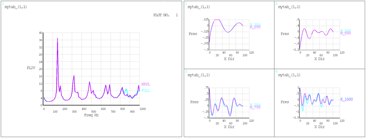
The resulting pressure wave animation, pressure distribution as a function of length, and frequency response function (FRF) of the system are presented in the figures below. The figures plotting results using both the Krylov and the full method show that their results are nearly equal.
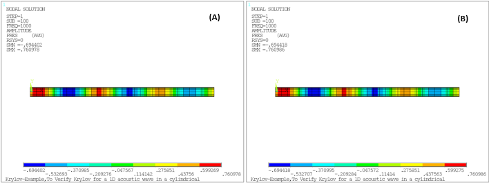
Figure 4.8: Pressure Distribution and Frequency Response Function (FRF): Krylov Compared to Full Method
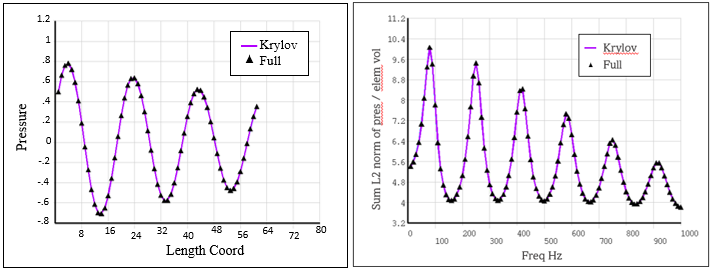
The presure distribution and the frequency response function (FRF)
calculated by the Krylov method are nearly identical to those calculated by the
full method. The peaks of the FRF correspond to the natural frequencies of the
system calculated in the modal analysis as seen in the following figure and
table.
Table 4.6: Natural Frequencies Computed in Modal Analysis
| Mode no. | Frequency (Hz) |
| 1 | 83 |
| 2 | 250 |
| 3 | 416 |
| 4 | 583 |
| 5 | 749 |
| 6 | 916 |
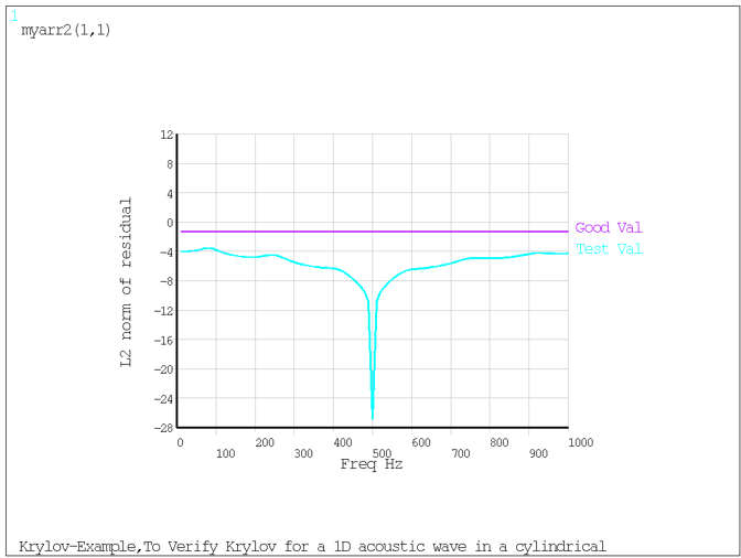
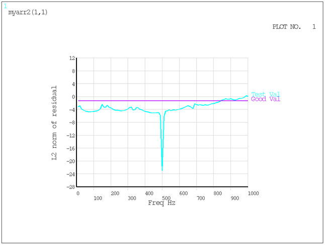
The following figure provides another measure of the accuracy of the solution.
The L2-norm of calculated residuals are below the acceptable tolerance
(RESTOL on KRYOPT) across the
entire frequency range.
/batch,list
/title, Krylov-Example,To Verify Krylov for a 1D acoustic wave in a cylindrical duct
/filname,Krylov-Example,1
/com
/com,*                   Model Details:
/com,  * The model is a acoustic duct with pressure load on 1 end and output impedance on other end
/com,*=======================================================================
/com,*                   TEST OBJECTIVES:
/com,*
/com,* To test the accuracy of Krylov for a 1D acoustic wave in a cylindrical duct
/com,*
/com,* The model is solved twice
/com,* Case-A  with FULL
/com,* Case-B  With Krylov
/com,*
/com,* EXPECTED result
/com,*
/com,* Krylov results match within 5% of full method
/com,*=======================================================================
/out,Krylov-Example-scratch,txt

/prep7
/units,mks

!!! Geo Details
pi = acos(-1)
rho = 1.2                        ! density
c0 = 340                         ! Speed of Sound
frq = 1000                       ! excitation freq   Hz
visco = 0.9                      ! viscosity

TP = 1/frq
WL = c0*TP
no_wl = 3                       ! no of wavelengths in space

cyl_L = no_wl*WL                 ! length of duct
cyl_r = 0.025*cyl_L              ! cross section of duct

nelem_wl = 10                    ! no of elements per wavelength
tol_elem = nelem_wl*no_wl

!!! Element & Matl definition

ET,1,fluid220
keyo,1,2,1          ! Uncoupled acoustic element without FSIs

MP,DENS,1,rho
MP,SONC,1,c0
mp,visc,1,visco

!!! Geometry creation

alls,all
csys,0
wpcsys,-1
wprota,,,90
asel,none
vsel,none
CYL4,,,cyl_r
wpcsys,-1
vext,all,,,cyl_L
VSBW,all,,DELETE
wprota,,90
VSBW,all,,DELETE
wpcsys,-1
cm,temp3_,volu

!!! Mesh Creation

mat,1
type,1

cmsel,s,temp3_
aslv
lsla
lsel,u,loc,x,0
lsel,u,loc,x,cyl_L
lesize,all,,,tol_elem
lsla
vsweep,all

/NUMBER,1
/PNUM,TYPE,1
alls,all
eplot

!!! LOAD & BC
cmsel,s,temp3_
aslv
asel,r,ext
asel,r,loc,x,0
nsla,s,1
D,ALL,pres,1

cmsel,s,temp3_
aslv
asel,r,ext
asel,r,loc,x,cyl_L
nsla,s,1
sf,all,impd,1000,

!!! Nodal array for post processing
nsel,s,loc,z,0
nsel,r,loc,y,0
esln
cm,elem_comp,elem
*get,count_,node,0,count
*dim,node_arr,array,count_,2
*dim, ordering,,count_
tmp_ = 0
*do,ii,1,count_
*get,tmp_,node,tmp_,nxth
node_arr(ii,1) = tmp_
*get,node_arr(ii,2),node,tmp_,loc,x
*enddo
*moper,ordering(1),node_arr(1,1),sort,,2

alls,all
cmsel,all
csys,0
finish

cdwrite,db,Krylov-Example,cdb
finish

!!!!!!!!!!!!!!!!!!!!!!!!!!!!!!!!!!!!!!!!!!!!!!!!!!!!!!!!!!!!!!!!!!!!!!!!
!!!!!!!!!!!!!!!!!!!!!!!!!!!!!!!!!!!! MODAL ANALYSIS
/clear,nostart
finish
cdread,db,Krylov-Example,cdb
finish

/solu
ANTYPE,Modal                       ! MODAL ANALYSIS
modopt,damp,12
SOLVE
FINISH

/post1
file,Krylov-Example,rst
set,last
set,list
*dim,eigen_,array,6,2
*do,ii,1,6
jj = 2*ii-1
eigen_(ii,1) = ii
*get,eigen_(ii,2),mode,jj,DFRQ
*enddo

/out
/com,
/com, *********  MODAL ANALYSIS TO LIST EIGEN VALUES
/com,
/com, Mode No.      Frequency
*vwrite,eigen_(1,1),eigen_(1,2)
(F8.0,'    |  ',F8.0)
/out,Krylov-Example-scratch,txt,,append
finish
!!!!!!!!!!!!!!!!!!!!!!!!!!!!!!!!!!!!!!!!!!!!!!!!!!!!!!!!!!!!!!!!!!!!!!!!
!!!!!!!!!!!!!!!!!!!!!!!!!!!!!!!!!!!! CASE -1 HARMONIC FULL METHOD

/clear,nostart
finish
cdread,db,Krylov-Example,cdb

/out,Krylov-Example-FULL-Echo,txt
/solu
ANTYPE,HARMIC                       ! HARMONIC ANALYSIS
HROPT,FULL                          ! FULL METHOD
EQSLV,SPARSE
HARFRQ,0,1000
nsub_ = 100
NSUB,nsub_
SOLVE
FINISH
/out,Krylov-Example-scratch,txt,,append

/post1
/edge,1,1
set,1,nsub_,,3,,60
/show,png,rev,,8
/graphics,power
/DSCALE,ALL,1.0
/PLOPTS,MINM,0
/PLOPTS,DATE,0
/plopts,info,3
/UDOC,1,DATE,0
/dev,font,1,Arial*Black
plnsol,pres
!anharm,20,0.1,10,-1
/show,close
/rename,Krylov-Example000,png,,Krylov-Example-FULL-PRES,png

!!!  Pressure as a func of Length Coord

*dim,res1_F,table,count_,2
res1_F(0,1) = 1

set,1,nsub_,,3,,60
*do,ii,1,count_
res1_F(ii,0) = ii
*get,res1_F(ii,1),node,node_arr(ii,1),pres
*enddo

!!! Sum of square of the L2 norm of pressure over element volume as a func of Freq

*dim,frq_arr,array,nsub_,1
*dim,res2_F,table,nsub_,2
res2_F(0,1)= 1

*do,jj,1,nsub_

set,1,jj,,3,,25

cmsel,s,elem_comp
nsle
*get,freq,active,,set,freq
etable,pl2fre,smisc,4
ssum
*get,pl2fres,SSUM,,ITEM,pl2fre
res2_F(jj,0) = freq
res2_F(jj,1) = sqrt(pl2fres)

frq_arr(jj) = freq
*enddo

parsav,all,Krylov-Example,param
fini
!!!!!!!!!!!!!!!!!!!!!!!!!!!!!!!!!!!!!!!!!!!!!!!!!!!!!!!!!!!!!!!!!!!!!!!!!!!!!!!!
!!!!!!!!!!!!!!!!!!!!!!!!!!!!!!!!!!!! CASE -2 HARMONIC KRYLOV METHOD

/clear,nostart
finish
cdread,db,Krylov-Example,cdb
parres,new,Krylov-Example,param

/out,Krylov-Example-KRYLOV-Echo,txt
/solu
ANTYPE,HARMIC                       ! HARMONIC ANALYSIS
resval_ = 0.05                      ! norm of residual for acceptable krylov result
/out
HROPT,krylov                        ! KRYLOV METHOD
kryopt,,,,resval_
/out,Krylov-Example-KRYLOV-Echo,txt,,append
EQSLV,SPARSE
HARFRQ,0,frq
NSUB,nsub_
SOLVE
FINISH
/out,Krylov-Example-scratch,txt,,append
!!!!!!!!!!!!!!!!!!!!!!!! To plot KRYLOV residuals

*dim,mystr1,string,248,1
mystr1(1) = UPCASE('  Frequency            L2 norm of residual')

*sread,mystr2,Krylov-Example-KRYLOV-Echo,txt,,248   !read file
*get,lines_,PARM,mystr2,dim,y                       !get length of file
line_ = 0
*do,ii,1,lines_
    *if,mystr1(1),eq,UPCASE(mystr2(1,ii)),then,     !compare desired string to file line
        line_=ii
		*exit                                      ! exit do loop
    *endif
*enddo

*dim,myarr1,array,nsub_,2
*vread,myarr1,Krylov-Example-KRYLOV-Echo,txt,,jik,2,nsub_,1,line_
(F22.6,F22.6)

*dim,myarr2,table,nsub_,2
myarr2(0,1) = 1
myarr2(0,2) = 2
*do,ijk,1,nsub_
myarr2(ijk,0) = myarr1(ijk,1)
myarr2(ijk,1) = log10(myarr1(ijk,2))
myarr2(ijk,2) = log10(resval_)
*enddo

/show,png,rev,,8
/PLOPTS,MINM,0
/PLOPTS,DATE,0
/PLOPTS,LOGO,1
/dev,font,1,Arial*Black
/gtype,all,grph,1
/axlab,X,'Freq Hz'
/axlab,Y,'L2 norm of residual'
/gcolumn,1,'Test Val'
/gcolumn,2,'Good Val'
*vplot,myarr2(1,0),myarr2(1,1),2
/show,close
/rename,Krylov-Example000,png,,Krylov-Example-KRYLOV-Residuals,png
!!!!!!!!!!!!!!!!!!!!!!!!!!!!!!!!!!!!!!!!!!!!!!!!!!!!!!!!!!!!!!!!!!!!!!!

/post1
/edge,1,1
set,1,nsub_,,3,,60
/show,png,rev,,8
/graphics,power
/DSCALE,ALL,1.0
/PLOPTS,MINM,0
/PLOPTS,DATE,0
/plopts,info,3
/UDOC,1,DATE,0
/dev,font,1,Arial*Black
plnsol,pres
!anharm,20,0.1,10,-1
/show,close
/rename,Krylov-Example000,png,,Krylov-Example-KRYLOV-PRES,png

!!!  Pressure as a func of Length Coord

set,1,nsub_,,3,,60
*do,ii,1,count_
*get,res1_F(ii,2),node,node_arr(ii,1),pres
*enddo

!!! Sum of square of the L2 norm of pressure over element volume as a func of Freq

*do,jj,1,nsub_

set,1,jj,,3,,25

cmsel,s,elem_comp
nsle
*get,freq,active,,set,freq
etable,pl2fre,smisc,4
ssum
*get,pl2fres,SSUM,,ITEM,pl2fre
res2_F(jj,2) = sqrt(pl2fres)
*enddo
finish

!!!!!!!!!!!!!!!!!!!!!!!!!!!!!!!!!!!!!!!!!!!!!!!!!!!!!!!!!!!!!!!!!!!!!!!!
!!!!!!!!!!!!!!!!!!!!!!!!!!!!!!!!!!!!!!!!!!!!!!!!!!!!!!!!!!!!!!!!!!!!!!!!
!!!!!!!!!!!!!!!!!!!!!!!!!!!!!!!!!!!!!!!!!!!!!!!!!!!!!!!!!!!!!!!!!!!!!!!!

!!! PLOTS

/show,png,rev,,8
/PLOPTS,MINM,0
/PLOPTS,DATE,0
/PLOPTS,LOGO,1
/dev,font,1,Arial*Black
/gtype,all,grph,1
/axlab,X,'Length Coord'
/axlab,Y,'Pressure'
/gcolumn,1,'Full'
/gcolumn,2,'Krylov'
/GMARKER,2,1
*vplot,res1_F(1,0),res1_F(1,1),2
/show,close
/rename,Krylov-Example000,png,,Krylov-Example-Pres-vs-Xcoord,png

/show,png,rev,,8
/PLOPTS,MINM,0
/PLOPTS,DATE,0
/PLOPTS,LOGO,1
/dev,font,1,Arial*Black
/gtype,all,grph,1
/axlab,X,'Freq Hz'
/axlab,Y,'Sum L2 norm of pres over elem vol'
/gcolumn,1,'Full'
/gcolumn,2,'Krylov'
/GMARKER,2,1
*vplot,res2_F(1,0),res2_F(1,1),2
/show,close
/rename,Krylov-Example000,png,,Krylov-Example-FRF,png


!!!!!!!!!!!!!!!!!!!!!!!!!!!!!!!!!!!!!!!!!!!!!!!!!!!!!!!!!!!!!!!!!!!!!!!!
!!!!!!!!!!!!!!!!!!!!!!!!!!!!!!!!!!!!!!!!!!!!!!!!!!!!!!!!!!!!!!!!!!!!!!!!
!!!!!!!!!!!!!!!!!!!!!!!!!!!!!!!!!!!!!!!!!!!!!!!!!!!!!!!!!!!!!!!!!!!!!!!!
/out,
/com,
/com,
/com, ********* COMPARING FULL AND KRYLOV (sum of Square of the L2 norm of pressure over element volume)
/com,           (FRF is attached which shows resonance)
/com,
/COM,  Freq      FULL      KRYLOV
/com
*VWRITE,res2_F(1,0),res2_F(1,1),res2_F(1,2)
(F8.2,'  ',F10.2,'   | ',F10.2)
/com,================================================================================
/com,
/com, ********* COMPARING FULL AND KRYLOV RESULTS Post1 results
/com,           (Harmonic response for last frequency)
/com,
/COM,NODE        FULL          KRYLOV
/com
*VWRITE,node_arr(1,1),res1_F(1,1),res1_F(1,2)
(F6.0,'   ',F10.2,'   | ',F10.2)
/com,================================================================================

/out,Krylov-Example-scratch,txt,,append
finish
/exit,nosav
Example 4.2: Krylov Harmonic Analysis of a 3D Piston Baffle Assembly Connected to a PML
This example problem demonstrates the use of the frequency-sweep Krylov method to simulate an acoustic geometry containing a pipe, which is connected to a piston at the inlet and the infinite baffle at the outlet. PML stimulates the infinite radition space. Results are compared to those obtained in a full harmonic analysis. The geometry is modeled with 220 elements.
Download the input file to run this example problem in batch mode: Krylov-Example2.dat (see command listing after results).
Results
Typical results such as pressure wave animation, pressure distribution as a function of length coordinate, and frequency response function (FRF) of the system are presented in the figures below. The figures plotting results using both the Krylov and the full method show that their results are closely related.
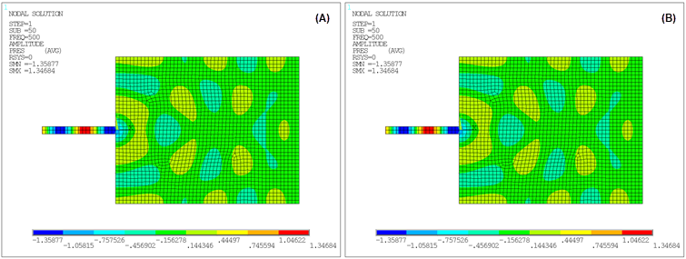
Figure 4.12: Frequency Response Function (FRF) and Path Plot of Pressure: Krylov Compared to Full Method for Four Distinct Frequency Points on the Spectrum
The following figure provides another measure of the accuracy of the solution.
The L2-norm of calculated residuals are below the acceptable tolerance
(RESTOL on KRYOPT) across the
0-800 Hz frequency range.
The following figure provides the Cartesian coordinate system plot of the acoustic far field parameter Sound Pressure Level (SPL dB) using both the Krylov method and the full method.
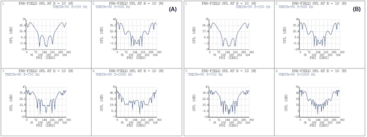
Observation – SPL plots
typically show a difference between the Krylov and full methods. Since far field
acoustic parameter plots require very high-fidelity simulations such as the full
method, the Krylov method is not a suitable option for these types of plots.
However, the Krylov method is a good candidate for obtaining high speed
simulations when looking at global system behavior (for example, FRF plots) to
help in quickly evaluating multiple design points of a model.
Command Listing
/batch,list
/title, Krylov-Example2,  Using Krylov method for acoustic PML
/com
/com,  * The model consists of a Geo modeled with 220 elements
/com,    Geo has piston at one end and an infinite baffle at another end
/com,    A sound-absorption material is located at the end of enclosure, modeled using PML.
/com,*=======================================================================

/out,scratch,txt

*get,jbnam,active,0,jobnam

!!! structure dimensions

/prep7
c0=340

d=0.1
l=1.
s=0.5
a=2

h=d/2
dpml=0.5

!!! define elements and material
et,11,200,7
et,1,220,,1           ! acoustic

et,2,220,,1,,1        ! pml

mp,dens,1,1.
mp,sonc,1,c0

!!! create GEo and Mesh
asel,none
rect,0,a,-a/2,a/2

rect,a,a+dpml,-a/2,a/2
alls,all
/PNUM,AREA,1
/PNUM,LINE,1
/NUMBER,0
aplot
alls,all
asel,u,area,,1
cm,tmp0,area
alls,all

asel,s,area,,1
cm,tmp1,area

alls,all
rect,-l,0,-d/2,d/2

aglue,all
wprota,,90
asbw,all,,dele
alls,all
wpcsys,-1,0
aplot

esize,h
type,11
amesh,all

mshape,0
mshkey,0
asel,u,area,,6,7
esla
type,1
mat,1
esize,,1
vext,all,,,0,0,d,

asel,s,area,,6,7
type,2,
mat,1
esize,,1
vext,all,,,0,0,d,

asel,s,loc,z,0
aclear,all
alls
nummrg,all

alls,all
/NUMBER,1
/PNUM,TYPE,1
eplot

!!! BC's
/prep7
lsclear,all

nsel,s,loc,x,a+dpml
nsel,a,loc,y,-a/2-dpml
nsel,a,loc,y,a/2+dpml
d,all,pres,0.

nsel,s,loc,x,-l
d,all,pres,1                 ! hard excitation source
alls

nsel,s,loc,x,a
esln
esel,r,type,,1
sf,all,mxwf
alls

!!! Result components
esel,all
nsel,s,loc,z,0
nsel,r,loc,y,0
nsel,r,loc,x,0,a+dpml
esln,r
*get,count_,node,0,count
cm,node_comp,node
cm,elem_comp,elem

*dim,node_arr,array,count_,2
*dim, ordering,,count_
tmp_ = 0
*do,ii,1,count_
*get,tmp_,node,tmp_,nxth
node_arr(ii,1) = tmp_
*get,node_arr(ii,2),node,tmp_,loc,x
*enddo
*moper,ordering(1),node_arr(1,1),sort,,2

alls,all
cmsel,all
csys,0
finish

cdwrite,db,%jbnam%,cdb
finish

!!!!!!!!!!!!!!!!!!!!!!!!!!!!!!!!!!!!!!!!!!!!!!!!!!!!!!!!!!!!!!!!!!!!!!!!!!!!!!!!!!!!!!!!!
!!!!!!!!!!!!!!!!!!!!!!!!!!!!!!!!!!!!!!!!!!!!!!!!!!!!!!!!!!!!!!!!!!!!!!!!!!!!!!!!!!!!!!!!!
!!!!!!!!!!!!!!!!!!!!!!!!!!!!!!!!!!!!!!!!!!!!!!!!!!!!!!!!!!!!!!!!!!!!!!!!!!!!!!!!!!!!!!!!!

        	!!!!!  TO GENERATE REF RESULTS - CASE -1 FULL METHOD

/clear,nostart
finish
*get,jbnam,active,0,jobnam
/prep7
cdread,db,%jbnam%,cdb

/gopr
/out,%jbnam%-FULL-ECHO,txt
/solu
ANTYPE,HARM                       ! HARMONIC ANALYSIS
HROPT,FULL                          ! FULL METHOD
nsub_ = 100
frq1=0
frq2=1000
phase_ = 30
HARFRQ,frq1,frq2
NSUB,nsub_
kbc,1
refl_coef = -40
pmlopt,0,three,refl_coef,refl_coef,refl_coef,refl_coef,refl_coef,refl_coef,prop,prop,prop,prop,prop,prop,
SOLVE
FINISH
/out,scratch,txt,,append

!!!!!!!!!!!!!!!!!!!!!!!!!!!!!!!!!!!!!!!!!!!!!!!!!!!!!!!!!!!!!!!!!!!!!!!
!!!  Pressure contour plots
!!!!!!!!!!!!!!!!!!!!!!!!!!!!!!!!!!!!!!!!!!!!!!!!!!!!!!!!!!!!!!!!!!!!!!!
/post1
file,%jbnam%,rst
/edge,1,1
/graphics,power
/DSCALE,ALL,1.0

no_freq = 4           ! total freq for post processsing
*dim,frq_post,array,4
frq_post(1) = 0.25*frq2,0.5*frq2,0.75*frq2,1*frq2

*do,pqr,1,no_freq
set,near,,,3,frq_post(pqr),phase_
*get,freq,active,,set,freq
/show,png,rev,,8
/graphics,power
/PLOPTS,MINM,0
/PLOPTS,DATE,0
/plopts,info,3
/UDOC,1,DATE,0
/dev,font,1,Arial*Black
plnsol,pres
!anharm,20,0.1,10,-1
/show,close
/rename,%jbnam%000,png,,%jbnam%-FULL-Pres-%freq%Hz,png
*enddo

!!!!!!!!!!!!!!!!!!!!!!!!!!!!!!!!!!!!!!!!!!!!!!!!!!!!!!!!!!!!!!!!!!!!!!!
!!! Far field Sound pressure level
!!!!!!!!!!!!!!!!!!!!!!!!!!!!!!!!!!!!!!!!!!!!!!!!!!!!!!!!!!!!!!!!!!!!!!!
alls,all
/show,png,
/graphics,power
/WIND,ALL,OFF
/WIND,1,ltop
/WIND,2,rtop
/WIND,3,lbot
/WIND,4,rbot
/gtype,all,grph,1
*do,ijk,1,no_freq
temp__ = frq_post(ijk)
set,near,,,0,temp__
/win,all,off
/win,ijk,on
/PLOPTS,MINM,0
/PLOPTS,DATE,0
/plopts,info,3
/UDOC,1,DATE,0
/PLOPTS,LOGO,0
plfar,pres,splc,0,360,360,90,90,1,10,2.e-5
/noerase
*enddo
/reset
/show,close
/rename,%jbnam%000,png,,%jbnam%-FULL-FARFIELD-SPL-vs-Phi,png

!!!!!!!!!!!!!!!!!!!!!!!!!!!!!!!!!!!!!!!!!!!!!!!!!!!!!!!!!!!!!!!!!!!!!!!
!!!    Store Response along a line
!!!!!!!!!!!!!!!!!!!!!!!!!!!!!!!!!!!!!!!!!!!!!!!!!!!!!!!!!!!!!!!!!!!!!!!
*dim,res1_F,table,count_,no_freq
*do,ii,1,no_freq
res1_F(0,ii) = ii
*enddo
*do,pqr,1,no_freq
set,near,,,3,frq_post(pqr),phase_
*do,ii,1,count_
res1_F(ii,0) = ii
*get,res1_F(ii,pqr),node,node_arr(ii,1),pres
*enddo
*enddo

!!!!!!!!!!!!!!!!!!!!!!!!!!!!!!!!!!!!!!!!!!!!!!!!!!!!!!!!!!!!!!!!!!!!!!!
!!!   Store FRF for Square of the L2 norm of pressure over element volume
!!!!!!!!!!!!!!!!!!!!!!!!!!!!!!!!!!!!!!!!!!!!!!!!!!!!!!!!!!!!!!!!!!!!!!!
*dim,frq_arr,array,nsub_,1
*dim,res2_F,table,nsub_,1
res2_F(0,1)= 1

*do,jj,1,nsub_
set,,,,,,,2*jj-1
*get,ls,active,0,set,lstp
*get,ss,active,0,set,sbst

set,ls,ss,,3,,phase_
etabl,erase
esel,s,type,,1
nsle
*get,freq,active,,set,freq
etable,pl2fre,smisc,4
ssum
*get,pl2fres,SSUM,,ITEM,pl2fre
res2_F(jj,0) = freq
res2_F(jj,1) = sqrt(pl2fres)

frq_arr(jj) = freq
*enddo

parsav,all,%jbnam%-FULL,param
!/exit,nosav

!!!!!!!!!!!!!!!!!!!!!!!!!!!!!!!!!!!!!!!!!!!!!!!!!!!!!!!!!!!!!!!!!!!!!!!!!!!!!!!!!!!!!!!!!
!!!!!!!!!!!!!!!!!!!!!!!!!!!!!!!!!!!!!!!!!!!!!!!!!!!!!!!!!!!!!!!!!!!!!!!!!!!!!!!!!!!!!!!!!
!!!!!!!!!!!!!!!!!!!!!!!!!!!!!!!!!!!!!!!!!!!!!!!!!!!!!!!!!!!!!!!!!!!!!!!!!!!!!!!!!!!!!!!!!

!!!! CASE -2 KRYLOV METHOD

/clear,nostart
finish
*get,jbnam,active,0,jobnam
/prep7
cdread,db,%jbnam%,cdb
parres,new,%jbnam%-FULL,param
resval_ = 0.05                      ! norm of residual for acceptable krylov result

/gopr
/out,
/solu
ANTYPE,HARM                       ! HARMONIC ANALYSIS
HARFRQ,frq1,frq2
NSUB,nsub_
HROPT,krylov                        ! KRYLOV METHOD
kryopt,120,,,resval_
kbc,1
pmlopt,0,three,refl_coef,refl_coef,refl_coef,refl_coef,refl_coef,refl_coef,prop,prop,prop,prop,prop,prop,
/out,%jbnam%-KRYL-ECHO,txt
SOLVE
FINISH
/out,scratch,txt,,append

!!!!!!!!!!!!!!!!!!!!!!!!!!!!!!!!!!!!!!!!!!!!!!!!!!!!!!!!!!!!!!!!!!!!!!!
!!! To plot KRYLOV residuals
!!!!!!!!!!!!!!!!!!!!!!!!!!!!!!!!!!!!!!!!!!!!!!!!!!!!!!!!!!!!!!!!!!!!!!!

*dim,mystr1,string,248,1
mystr1(1) = UPCASE('  Frequency            L2 norm of residual')

*sread,mystr2,%jbnam%-KRYL-ECHO,txt,,248   !read file
*get,lines_,PARM,mystr2,dim,y                       !get length of file
line_ = 0
*do,ii,1,lines_
    *if,mystr1(1),eq,UPCASE(mystr2(1,ii)),then,     !compare desired string to file line
        line_=ii
		*exit                                      ! exit do loop
    *endif
*enddo

*dim,myarr1,array,nsub_,2
*vread,myarr1,%jbnam%-KRYL-ECHO,txt,,jik,2,nsub_,1,line_
(F22.6,F22.6)

*dim,myarr2,table,nsub_,2
myarr2(0,1) = 1
myarr2(0,2) = 2
*do,ijk,1,nsub_
myarr2(ijk,0) = myarr1(ijk,1)
myarr2(ijk,1) = log10(myarr1(ijk,2))
myarr2(ijk,2) = log10(resval_)
*enddo

/show,png,rev,,8
/PLOPTS,MINM,0
/PLOPTS,DATE,0
/PLOPTS,LOGO,1
/dev,font,1,Arial*Black
/gtype,all,grph,1
/axlab,X,'Freq Hz'
/axlab,Y,'L2 norm of residual'
/gcolumn,1,'Test Val'
/gcolumn,2,'Good Val'
*vplot,myarr2(1,0),myarr2(1,1),2
/show,close
/rename,%jbnam%000,png,,%jbnam%-KRYL-Residuals,png

!!!!!!!!!!!!!!!!!!!!!!!!!!!!!!!!!!!!!!!!!!!!!!!!!!!!!!!!!!!!!!!!!!!!!!!
!!!  Pressure contour plots
!!!!!!!!!!!!!!!!!!!!!!!!!!!!!!!!!!!!!!!!!!!!!!!!!!!!!!!!!!!!!!!!!!!!!!!
/post1
file,%jbnam%,rst
/edge,1,1
/graphics,power
/DSCALE,ALL,1.0

*do,pqr,1,no_freq
set,near,,,3,frq_post(pqr),phase_
*get,freq,active,,set,freq
/show,png,rev,,8
/graphics,power
/PLOPTS,MINM,0
/PLOPTS,DATE,0
/plopts,info,3
/UDOC,1,DATE,0
/dev,font,1,Arial*Black
plnsol,pres
/show,close
/rename,%jbnam%000,png,,%jbnam%-KRYL-Pres-%freq%Hz,png
*enddo

!!!!!!!!!!!!!!!!!!!!!!!!!!!!!!!!!!!!!!!!!!!!!!!!!!!!!!!!!!!!!!!!!!!!!!!
!!! Far field Sound pressure level
!!!!!!!!!!!!!!!!!!!!!!!!!!!!!!!!!!!!!!!!!!!!!!!!!!!!!!!!!!!!!!!!!!!!!!!
alls,all
/show,png,
/graphics,power
/WIND,ALL,OFF
/WIND,1,ltop
/WIND,2,rtop
/WIND,3,lbot
/WIND,4,rbot
/gtype,all,grph,1
*do,ijk,1,no_freq
temp__ = frq_post(ijk)
set,near,,,0,temp__
/win,all,off
/win,ijk,on
/PLOPTS,MINM,0
/PLOPTS,DATE,0
/plopts,info,3
/UDOC,1,DATE,0
/PLOPTS,LOGO,0
plfar,pres,splc,0,360,360,90,90,1,10,2.e-5
/noerase
*enddo
/reset
/show,close
/rename,%jbnam%000,png,,%jbnam%-KRYL-FARFIELD-SPL-vs-Phi,png

!!!!!!!!!!!!!!!!!!!!!!!!!!!!!!!!!!!!!!!!!!!!!!!!!!!!!!!!!!!!!!!!!!!!!!!
!!!  Store Response along a line
!!!!!!!!!!!!!!!!!!!!!!!!!!!!!!!!!!!!!!!!!!!!!!!!!!!!!!!!!!!!!!!!!!!!!!!
*dim,res1_K,table,count_,no_freq
*do,ii,1,no_freq
res1_K(0,ii) = ii
*enddo
*do,pqr,1,no_freq
set,near,,,3,frq_post(pqr),phase_
*do,ii,1,count_
res1_K(ii,0) = ii
*get,res1_K(ii,pqr),node,node_arr(ii,1),pres
*enddo
*enddo

!!!!!!!!!!!!!!!!!!!!!!!!!!!!!!!!!!!!!!!!!!!!!!!!!!!!!!!!!!!!!!!!!!!!!!!
!!!   Store FRF for Square of the L2 norm of pressure over element volume
!!!!!!!!!!!!!!!!!!!!!!!!!!!!!!!!!!!!!!!!!!!!!!!!!!!!!!!!!!!!!!!!!!!!!!!
*dim,frq_arr,array,nsub_,1
*dim,res2_K,table,nsub_,1
res2_K(0,1)= 1

*do,jj,1,nsub_
set,,,,,,,2*jj-1
*get,ls,active,0,set,lstp
*get,ss,active,0,set,sbst

set,ls,ss,,3,,phase_
etabl,erase
esel,s,type,,1
nsle
*get,freq,active,,set,freq
etable,pl2fre,smisc,4
ssum
*get,pl2fres,SSUM,,ITEM,pl2fre
res2_K(jj,0) = freq
res2_K(jj,1) = sqrt(pl2fres)

frq_arr(jj) = freq
*enddo

!!!!!!!!!!!!!!!!!!!!!!!!!!!!!!!!!!!!!!!!!!!!!!!!!!!!!!!!!!!!!!!!!!!!!!!!!!!!!!!!!!!!!!!!!
!!!!!!!!!!!!!!!!!!!!!!!!!!!!!!!!!!!!!!!!!!!!!!!!!!!!!!!!!!!!!!!!!!!!!!!!!!!!!!!!!!!!!!!!!
!!!!!!!!!!!!!!!!!!!!!!!!!!!!!!!!!!!!!!!!!!!!!!!!!!!!!!!!!!!!!!!!!!!!!!!!!!!!!!!!!!!!!!!!!

!!!!!!!!!          PLOTS

!!!!!!!!!!!!!!!!!!!!!!!!!!!!!!!!!!!!!!!!!!!!!!!!!!!!!!!!!!!!!!!!!!!!!!!
!!!  PLOT Response along a line
!!!!!!!!!!!!!!!!!!!!!!!!!!!!!!!!!!!!!!!!!!!!!!!!!!!!!!!!!!!!!!!!!!!!!!!

/show,png,rev,,8
/graphics,power
/axlab,X,X Dir
/axlab,Y,Pres
/WIND,ALL,OFF
/WIND,1,ltop
/WIND,2,rtop
/WIND,3,lbot
/WIND,4,rbot
/gtype,all,grph,1

*do,ijk,1,no_freq
temp__ = frq_post(ijk)
temp__ = nint(temp__)
*del,mytab_
*dim,mytab_,table,count_,2

*do,pqr,1,count_
mytab_(pqr,0) = pqr
mytab_(pqr,1) = res1_F(pqr,ijk)
mytab_(pqr,2) = res1_K(pqr,ijk)
*enddo

/win,all,off
/win,ijk,on
/PLOPTS,MINM,0
/PLOPTS,DATE,0
/plopts,info,3
/UDOC,1,DATE,0
/PLOPTS,LOGO,0
/dev,font,1,Arial*Black
/gcolumn,1,F_%temp__%
/gcolumn,2,K_%temp__%
*vplot,mytab_(1,0),mytab_(1,1),2
/noerase
*enddo
/reset
/show,close
/rename,%jbnam%000,png,,%jbnam%-RESP,png

!!!!!!!!!!!!!!!!!!!!!!!!!!!!!!!!!!!!!!!!!!!!!!!!!!!!!!!!!!!!!!!!!!!!!!!
!!!   PLOT FRF for Square of the L2 norm of pressure over element volume
!!!!!!!!!!!!!!!!!!!!!!!!!!!!!!!!!!!!!!!!!!!!!!!!!!!!!!!!!!!!!!!!!!!!!!!

*del,mytab_
*dim,mytab_,table,nsub_,2
*do,ijk,1,nsub_
temp__ = frq_arr(ijk)
mytab_(ijk,0) = temp__
mytab_(ijk,1) = res2_F(temp__,1)
mytab_(ijk,2) = res2_K(temp__,1)
*enddo

/show,png,rev,,8
/axlab,X,Freq Hz
/axlab,Y,PL2V
/gcolumn,1,FULL
/gcolumn,2,KRYL
*vplot,mytab_(1,0),mytab_(1,1),2
/show,close
/rename,%jbnam%000,png,,%jbnam%-FRF,png

finish
/exit,nosav
Three Ansys Parametric Design Language (APDL) macros are available as templates that you can use to create a custom frequency-sweep harmonic analysis using the Krylov method. You can download them from the following links:
| KRYGENSUB.mac creates the Krylov subspace. (download) |
| KRYSOLVE.mac solves the reduced system of equations. (download) |
| KRYEXPAND.mac expands the Krylov subspace. (download) |
These macros must be run consecutively.
The theory demonstrated in these macros stems from the work of Puri, S. [1] and Eser, M. [2]. Although you can see all details of the Krylov approximation in the macros, it is worth noting the following assumptions inherent in the Krylov solution obtained using the unmodified macros:
The stiffness, mass, and damping matrices are assumed to be constant (independent of frequency).
The external load vector is linearly ramped over frequency. Ramping assumes that the frequency at which the Krylov subspace is built is in the middle of the frequency range. If you wish to apply stepped loading, there is an option to specify that in the inputs for the KRYSOLVE.mac macro.
The following sections describe and list the macros and the required and optional input values that you can modify to specify your analysis and provide an example problem and references for further information on the Krylov method.
For detailed information on APDL scripting to customize macros, see the Ansys Parametric Design Language Guide.
To implement the customizable Krylov method using the Python programming language, see Harmonic analysis using the Krylov method in the PyMAPDL User Guide
.
Caution: As with other user-programmable features, modifying these macros is a nonstandard use of the program that the Ansys, Inc. Quality Assurance verification testing program does not cover. You are responsible for verifying that the results produced are accurate and that the routines you link do not adversely affect other, standard areas of the program.
The first macro, KRYGENSUB.mac, generates a Krylov subspace used to reduce the FEA model in a harmonic analysis. The subspace is built using the assembled stiffness, mass, and damping matrices along with the load vector that must be present on a Jobname.full file located in your working directory. The following snippet shows how to generate the Jobname.full file with the matrices and load vector in the proper form for use by the KRYGENSUB.mac macro. To create the Jobname.full file using the snippet below, you must use shared-memory parallel (SMP) processing.
Example 4.3: Generate Jobname.full for Krylov method using Mechanical APDL
/PREP7

! Add commands here to generate the FEA model (mesh, constraints, loads, etc.)
...
...
...

/SOLU
ANTYPE,HARMIC
HROPT,KRYLOV         ! Required to write the .full file in proper format for Krylov subspace generation
!–––-Perform analysis from 300-700 Hz in 5 Hz increments-----
HARFRQ,300,700       ! Set the frequency range of interest
NSUBST,80            ! Set the number of frequency increments
WRFULL,1             ! Generate .full file and stop
SOLVE
FINI
Alternatively, you can import the required matrices and load vector from another source. To do so, modify the KRYGENSUB.mac to avoid reading the .full file and instead use the provided APDL Math parameters. For details on importing matrices and vectors from external sources, see Procedure for Using APDL Math in the Ansys Parametric Design Language Guide.
Required inputs for KRYGENSUB.mac — In addition to the required .full file, you must define the following input values in the macro to specify your problem:
The maximum size or dimension of the subspace (
maxDimQ). Larger values typically result in a more accurate solution but also require more computational effort to build and use the subspace to compute the final solution.The frequency value at which to build the subspace (
freqVal). This value is typically recommended to be in the middle of the frequency range.An optional key specifying whether or not to check if each subspace vector is orthonormal to all of the other vectors in the subspace (
chkOrthoKey). This one-time check is performed after the subspace has been generated and adds to the overall computational cost.An optional key to output the Kyrlov subspace to the Qz.txt file (
outKey).
!COM ************************************************************************
!COM KRYGENSUB.MAC                                                          *
!COM                                                                        *
!COM   This macro generates a Krylov subspace used for a model reduction    *
!COM   solution in a harmonic analysis. The subspace is built using the     *
!COM   assembled matrices and load vector on the jobname.full file that     *
!COM   is located in the current working directory.  This .full file        *
!COM   should be built at the specified frequency value.                    *
!COM                                                                        *
!COM   COMMAND USAGE: KRYGENSUB,maxDimQ,freqVal,chkOrthoKey,outKey          *
!COM     maxDimQ     - maximum size/dimension of Krylov subspace            *
!COM     freqVal     - frequency value (Hz) at which to build the KRYLOV    *
!COM                   subspace                                             *
!COM     chkOrthoKey - [optional] key to check orthonormal properties of    *
!COM                   each subspace vector with all other subspace vectors *
!COM     outKey      - [optional] key to output KRYLOV subspace to Qz.txt   *
!COM                   file                                                 *
!COM                                                                        *
!COM ************************************************************************

!Store input arguments from user
maxDimQ=arg1
freqVal=arg2
chkOrthoKey=arg3
outKey=arg4

!Check for illegal input values by user
*IF,maxDimQ,LE,0,THEN
  *msg,error
  The maximum size of Krylov subspace is required to be greater than 0
  _nerr=1
*ENDIF
*IF,freqVal,LT,0.0,THEN
  *msg,error
  The frequency value for building the Krylov subspace is required to be greater or equal to 0 Hz
  _nerr=1
*ENDIF
*IF,chkOrthoKey,LT,0,THEN
  *msg,error
  The chkOrthoKey value for building the Krylov subspace is required to be 0 or 1
  _nerr=1
*ENDIF
*IF,chkOrthoKey,GT,1,THEN
  *msg,error
  The chkOrthoKey value for building the Krylov subspace is required to be 0 or 1
  _nerr=1
*ENDIF
*IF,outKey,LT,0,THEN
  *msg,error
  The outKey value for building the Krylov subspace is required to be 0 or 1
  _nerr=1
*ENDIF
*IF,outKey,GT,1,THEN
  *msg,error
  The outKey value for building the Krylov subspace is required to be 0 or 1
  _nerr=1
*ENDIF


!Execute macro if no errors above
*IF,_nerr,EQ,0,THEN

!The coefficient to mass matrix term
twoPi=2.0*acos(-1)
omega0=freqVal*twoPi              !circular frequency at given frequency point
ccf=-omega0*omega0

!Make up full file name parameter
*GET,jobname1,ACTIVE,,jobname,,START,1
*GET,jobname2,ACTIVE,,jobname,,START,9
*GET,jobname3,ACTIVE,,jobname,,START,17
*GET,jobname4,ACTIVE,,jobname,,START,25
*SET,thejob,'%jobname1%%jobname2%%jobname3%%jobname4%'
*SET,fullfile,'%thejob%.full'

!Load global matrices and RHS in full file
*SMAT,MatK,D,IMPORT,FULL,fullfile,STIFF        !stiffness matrix [MatK]
*INQ,MatK,DIM2,nDOF                            !the 2nd matrix dimension,nDOF
*SMAT,MatM,D,IMPORT,FULL,fullfile,MASS         !mass matrix [MatM]
*SMAT,MatC,D,IMPORT,FULL,fullfile,DAMP         !damping matrix [MatC]
*SMAT,Nod2Solv,D,IMPORT,FULL,fullfile,NOD2SOLV !import the mapping vector
*VEC,Fz,Z,IMPORT,FULL,fullfile,RHS             !right hand side {Fz}
*VEC,Fz0,Z,COPY,Fz

!Form Az=(K-w0*w0*M,i*w0*C) and Cz=(C,i*2*w0*M)
*SMAT,Az,Z,COPY,MatK                           ![Az]=[MatK]
*AXPY,ccf,0.0,MatM,1.0,0.0,Az                  ![Az]=(1,0)*[Az]+(ccf,0)*[MatM]
*AXPY,0.0,omega0,MatC,1.0,0.0,Az               ![Az]=(1,0)*[Az]+(0,omega0)*[MatC]
*SMAT,Cz,Z,COPY,MatC                           ![Cz]=[MatC]
*AXPY,0.0,2.0*omega0,MatM,1.0,0.0,Cz           ![Cz]=(1,0)*[Cz]+(0,2*omega0)*[MatM]
zeroC=0                                        !set zeroC flag
*NRM,Cz,NRM2,normC,NO
*IF,normC,EQ,0.0,THEN
  zeroC=1
*ENDIF

!Solve for the 1st vector of subspace [Q]
*LSENGINE,DSP,DSPsolver,Az,INCORE              !create solver system of [Az]
*LSFACTOR,DSPsolver                            !factor [Az]
*DMAT,Qz,Z,ALLOC,nDOF,maxDimQ,INCORE           ![Qz] initially allocated
*VEC,Uz1,Z,LINK,Qz,1                           !{Uz1} linked to Qz[1]
*LSBAC,DSPsolver,Fz,Uz1                        !backward solve -> {Uz1}
*NRM,Uz1,NRM2,normU,YES                        !{Uz1} normalized

i1=2                                           !initialized as no damping
*IF,zeroC,EQ,0,THEN
  i1=3
  *VEC,Uz2,Z,LINK,Qz,2                         !{Uz2} linked to Qz[2]
  *INIT,Fz,ZERO                                !{Fz}=0
  *MULT,Cz,,Uz1,,Fz                            !{Fz}={Fz}+[Cz]{Uz1}
  *AXPY,0.0,0.0,Fz,-1.0,0.0,Fz                 !{Fz}=-{Fz}
  *NRM,Fz,NRM2,normU,YES
  *LSBAC,DSPsolver,Fz,Uz2                      !back solved:{Uz2}=[Az]^-1*{Fz}
  *DOT,Uz1,Uz2,ccon_real,ccon_imag             !{Uz2}*{v1} = ccon
  *AXPY,-ccon_real,-ccon_imag,Uz1,1.0,0.0,Uz2  !{Uz2}={Uz2}-ccon*{Uz1}
  *NRM,Uz2,NRM2,normU,YES                      !{Uz2} normalized
*ENDIF

!Build Subspace Vectors with MGS (2nd Order)
*DO,dimQ,i1,maxDimQ
  *IF,normU,EQ,0.0,THEN
    numQ=dimQ-1                                !exhausted at dimQ
  *ELSE
    numQ=maxDimQ                               !may reach to the maximum
  *ENDIF
  *IF,numQ,GE,maxDimQ,THEN                     !make next vector
    *INIT,Fz,ZERO
    *IF,zeroC,EQ,0,THEN                        ![Cz]!=0 case
      *SET,nextUzOne,dimQ-2
      *SET,nextUzTwo,dimQ-1
      *VEC,Uz1,Z,LINK,Qz,nextUzOne             !{Uz1} to [Qz](dimQ-2)
      *VEC,Uz2,Z,LINK,Qz,nextUzTwo             !{Uz2} to [Qz](dimQ-1)
      *VEC,Uz,Z,LINK,Qz,dimQ                   !{Uz} to [Qz](dimQ)
      *MULT,Cz,,Uz2,,Uz                        ![Cz]{Uz2} -> {Uz}
    *ELSE
      *SET,nextUzOne,dimQ-1                    ![Cz]=0 case
      *VEC,Uz1,Z,LINK,Qz,nextUzOne
      *VEC,Uz,Z,LINK,Qz,dimQ                   !{Uz} to [Qz](dimQ)
      *INIT,Uz,ZERO
    *ENDIF
    *MULT,MatM,,Uz1,,Fz                        ![MatM]{Uz1} -> {Fz}
    *AXPY,-1.0,0.0,Uz,-1.0,0.0,Fz              !{Fz} = -{Fz}-{Uz}
    *LSBAC,DSPsolver,Fz,Uz                     ![Az]^-1{Fz} -> {Uz}

    !Make subspace vectors orthonormal (MGS)
    *DO,j,1,dimQ-1
      *VEC,V1,Z,LINK,Qz,j
      *DOT,V1,Uz,ccon_real,ccon_imag
      *AXPY,-ccon_real,-ccon_imag,V1,1.,0.,Uz
    *ENDDO
    *NRM,Uz,NRM2,normU,YES                     !normalize {Uz}
  *ENDIF
*ENDDO

!Optional check on Orthonormality of vectors
*IF,chkOrthoKey,EQ,1,THEN
  *DO,i,1,numQ
    *VEC,Vz,Z,LINK,Qz,i
    *DO,j,1,numQ
      *VEC,Uz,Z,LINK,Qz,j
      *DOT,Vz,Uz,ccon_real,ccon_imag
      dcon=sqrt(ccon_real*ccon_real+ccon_imag*ccon_imag)
      *vwrite,i,j,dcon
      (' V_',F3.0,'V_',F3.0,' = ',E22.15,',',E22.15'i')
    *ENDDO
  *ENDDO
*ENDIF

!Output generated subspace vectors to file
*IF,outKey,EQ,1,THEN                           !output subspace vectors
  *PRINT,Qz,%thejob%_Qz.txt
*ENDIF

*ENDIF
/gopr
The second macro, KRYSOLVE.mac, uses the given Krylov subspace to reduce the system of equations. Once that step is complete, the macro loops over the frequency points in the given frequency range to compute the reduced solution.
Required inputs for KRYSOLVE.mac — You must execute KRYGENSUB.mac before running KRYSOLVE.mac. In addition, define the following input values in the macro to specify your analysis:
The beginning (
freqBeg) and end (freqEnd) points of the frequency range you wish to analyze.The number of frequency points at which to compute the harmonic solution (
numFreq).Specify whether the load is ramped or stepped by setting
loadKey= 0 or 1, respectively. If you do not specify a value forloadKey, the default is ramped (0 or blank). Generally, ramped loading is used for structural applications and stepped loading is recommended for acoustics analyses.An optional key to output the reduced solution to the Yz.txt file (
outKey).
!COM *****************************************************************************
!COM KRYSOLVE.MAC                                                                *
!COM                                                                             *
!COM  This macro uses a KRYLOV subspace to solve a reduced harmonic              *
!COM  analysis over a specified frequency range for a given number of            *
!COM  frequency points (intervals).                                              *
!COM                                                                             *
!COM  COMMAND USAGE: KRYSOLVE,freqBeg,freqEnd,numFreq,outKey                     *
!COM    freqBeg - starting value of the frequency range (Hz)                     *
!COM    freqEnd - ending value of the frequency range (Hz)                       *
!COM    numFreq - user specified number of intervals in frequency range          *
!COM    loadKey - key specifying whether load should be ramped(0) or stepped(1)  *
!COM    outKey  - [optional] key to output reduced solution to Yz.txt file       *
!COM                                                                             *
!COM *****************************************************************************

!Store input arguments from user
freqBeg=arg1
freqEnd=arg2
numFreq=arg3
loadKey=arg4
outKey=arg5

!Check for illegal input values by user
*IF,freqBeg,LT,0.0,THEN
  *msg,error
  The beginning frequency value for solving the reduced solution is required to be greater than or equal to 0
  _nerr=1
*ENDIF
*IF,numFreq,LE,0,THEN
  *msg,error
  The number of frequencies for which to compute the reduced solution is required to be greater than 0
  _nerr=1
*ENDIF
*IF,loadKey,LT,0,THEN
  *msg,error
  The loadKey value for computing the reduced solution is required to be 0 or 1
  _nerr=1
*ENDIF
*IF,loadKey,GT,1,THEN
  *msg,error
  The loadKey value for computing the reduced soluion is required to be 0 or 1
  _nerr=1
*ENDIF
*IF,outKey,LT,0,THEN
  *msg,error
  The outKey value for computing the reduced solution is required to be 0 or 1
  _nerr=1
*ENDIF
*IF,outKey,GT,1,THEN
  *msg,error
  The outKey value for computing the reduced soluion is required to be 0 or 1
  _nerr=1
*ENDIF


!Execute macro if no errors above
*IF,_nerr,EQ,0,THEN

!Define solution variables
*INQ,Az,DIM2,nDOF
*VEC,QtF,Z,ALLOC,dimQ                   !{QtF}, force vector in subspace
*DMAT,QtAQ,Z,ALLOC,dimQ,dimQ,INCORE     ![QtAQ], reduced matrix
*DMAT,Yz,Z,ALLOC,dimQ,numFreq,INCORE    ![Yz], reduced solution over range
*DMAT,QtA,Z,ALLOC,nDOF,dimQ,INCORE      ![QtA]
*DMAT,DzV,Z,ALLOC,nDOF,numFreq,INCORE   !{DzV}, displacement vector
*VEC,iRHS,Z,ALLOC,nDOF

!Loop over frequency range
*SET,omega,freqBeg*twoPi                !circular frequency at starting point
*SET,intV,(freqEnd-freqBeg)/numFreq
*DO,iFreq,1,numFreq
  !form RHS at the i-th freqency point
  *INIT,iRHS,ZERO                       !{iRHS}=0
  *IF,loadKey,eq,0,then
    !apply ramped loading
    *SET,ratio,2*iFreq/numFreq
    *IF,numFreq,EQ,1,THEN
      *SET,ratio,1.0d0
    *ENDIF
  *ELSE
     !apply stepped loading
     *SET,ratio,1.0d0
  *ENDIF
  *AXPY,ratio,0.0,Fz0,1.0,0.0,iRHS      !get {iRHS} at iFreq
  *MULT,Qz,TRANS,iRHS,,QtF              !reduce [Qz]^t{iRHS} -> {QtF}
  *VEC,iY,Z,LINK,Yz,iFreq               !link iY to Yz(iFreq)

  !Reduced system at omega
  *SET,omega,omega+intV*twoPi           !defined frequency value
  *SET,ccf,-omega*omega
  *SMAT,Az,Z,COPY,MatK                  !modified K:[Az]=[MatK]
  *AXPY,ccf,0.0,MatM,1.0,0.0,Az         ![Az]=(1,0)*[Az]+(ccf,0)*[MatM]
  *AXPY,0.0,omega,MatC,1.0,0.0,Az       ![Az]=(1,0)*[Az]-(0,omega)*[MatC]
  *MULT,Az,,Qz,,AQ                      ![AQ]=[Az][Qz]
  *MULT,Qz,TRANS,AQ,,QtAQ               ![QtAQ]=[Q^t][AQ]

  *LSENGINE,LAPACK,LAsolver,QtAQ,INCORE !create reduced system of equations
  *LSFACTOR,LAsolver                    !factor [QtAQ]
  *LSBAC,LAsolver,QtF,iY                !back solve for {iY}=Yz[iFreq]

  !Output reduced solution (if requested)
  *IF,outKey,EQ,1,THEN
    *PRINT,iY,'%thejob%_Yz_%iFreq%.txt' !Yz_*.txt, reduced solution vector
  *ENDIF
*ENDDO

*ENDIF
The third macro, KRYEXPAND.mac, expands the reduced solution at all frequency points in the given frequency range specified by the user back to the FEA model. When this macro is completed, the expanded solution can be output. You can also choose to compute the L-inf, L-1, or L-2 norm of the residual and output this quantity to provide a sense of the overall accuracy of the expanded solution, but norm computation at every frequency point adds to the overall computation time.
Required inputs for KRYEXPAND.mac — You must execute the first two macros, KRYGENSUB.mac and KRYSOLVE.mac, before running KRYEXPAND.mac. In addition, define the following input values in the macro to specify the residual of the expansion and write the expanded solution to a text file:
An optional key to output the expanded solution to the Xz_*.txt file (
outKey).An optional key to specify the computation of the residual of the expanded solution (
resKey). Possible settings are:0 - Do not compute the residual. 1 - Compute the L-inf norm of the residual. 2 - Compute the L-1 norm of the residual. 3 - Compute the L-2 norm of the residual.
Note that the final expanded solution at each frequency is written to the
Xz_*.txt files in the same ordering as the matrices
and load vector inputs to the KRYGENSUB.mac macro. If you
are using Mechanical APDL to generate the matrices and load vector, the node ordering
is defined by the process shown in Example 4.3: Generate Jobname.full for Krylov method using
Mechanical APDL. If,
instead, you are supplying the required matrices and load vector from an
external source, the expanded solution(s) will be output in the same ordering as
the given matrices and load vector.
!COM ***********************************************************************
!COM KRYEXPAND.MAC                                                         *
!COM                                                                       *
!COM   This macro expands the reduced solution for a harmonic analysis     *
!COM   back to the original space.  Optional calculation of the residual   *
!COM   is available.  Note, when this macro is finished all APDL Math      *
!COM   parameters will be deleted via the *FREE,ALL command.               *
!COM                                                                       *
!COM   COMMNAD USAGE: KRYEXPAND,outKey,resKey                              *
!COM     outKey  - [optional] key to output expanded solution to Xz_*.txt  *
!COM               file                                                    *
!COM     resKey  - [optional] key to compute the residual of the expanded  *
!COM               solution                                                *
!COM               = 0 means do not compute the residual                   *
!COM               = 1 means compute the L-inf norm of the residual        *
!COM               = 2 means compute the L-1 norm of the residual          *
!COM               = 3 means compute the L-2 norm of the residual          *
!COM                                                                       *
!COM ***********************************************************************

!Store input arguments from user
outKey=arg1
resKey=arg2

!Check for illegal input values by user
*IF,outKey,LT,0,THEN
  *msg,error
  The outKey value for expanding the reduced solution is required to be 0 or 1
  _nerr=1
*ENDIF
*IF,outKey,GT,1,THEN
  *msg,error
  The outKey value for expanding the reduced soluion is required to be 0 or 1
  _nerr=1
*ENDIF
*IF,resKey,LT,0,THEN
  *msg,error
  The resKey value for expanding the reduced solution is required to be 0 -> 3
  _nerr=1
*ENDIF
*IF,outKey,GT,3,THEN
  *msg,error
  The resKey value for expanding the reduced soluion is required to be 0 -> 3
  _nerr=1
*ENDIF


!Execute macro if no errors above
*IF,_nerr,EQ,0,THEN

*DMAT,RzV,Z,ALLOC,nDOF,1,INCORE

!Build mapping vectors
*VEC,MapForward,I,IMPORT,FULL,fullfile,FORWARD
*VEC,MapBack,I,IMPORT,FULL,fullfile,BACK
*INQ,MapForward,DIM1,MAXNODE
*INQ,MapBack,DIM1,NUMNODE

!Expand reduced solution
*SET,omega,freqBeg*twoPi                   !circular frequency at starting point
*DO,iFreq,1,numFreq
  *VEC,iY,Z,LINK,Yz,iFreq
  *VEC,Xi,Z,LINK,DzV,iFreq                 !vector of solution in solver space
  *INIT,Xi,ZERO
  *DO,jVect,1,dimQ                         !collect each vector's contribution
    *VEC,Qzj,Z,LINK,Qz,jVect               !link to the jVect-th vector
    yrj = iY(jVect,1)                      !real part of reduced solution
    yij = iY(jVect,2)                      !imaginary part of reduced solution
    *AXPY,yrj,yij,Qzj,1.0,0.0,Xi           !{Xi} = {Xi} + (yrj,yri)*{Qzj}
  *ENDDO

  !Output solution vectors (if requested)
  *IF,outKey,EQ,1,THEN
    *MULT,Nod2Solv,TRAN,Xi,,Xii            !Map {Xi} to internal (ANSYS) order

    !Map {Xii} to user ordering
    *INQ,Xii,DIM1,NUMEQN
    NUMDOF = NUMEQN/NUMNODE
    *CFOPEN,%thejob%_Xzu_%iFreq%,txt,,     !Write to Xiu_*.txt in user ordering
    *DO,extNode,1,MAXNODE
      intNode = MapForward(extNode)
      *IF,intNode,LE,0,THEN                !Skip nodes not mapped
         *CYCLE
      *ENDIF
      intEqn = (intNode-1)*NUMDOF
      extEqn = (extNode-1)*NUMDOF
      *DO,idof,1,NUMDOF
        Xii_real = Xii(intEqn+idof,1)      !Real value
        Xii_imag = Xii(intEqn+idof,2)      !Image value
        *vwrite,extNode,extEqn+idof,Xii_real,Xii_imag
        ('Node#=',F9.0,', Eqn#=',F9.0,', X=',E23.15,E23.15)
      *ENDDO
    *ENDDO
    *CFCLOS
    *PRINT,Xi,%thejob%_Xz_%iFreq%.txt      !internal solver space, Xz_*.txt
    *PRINT,Xii,%thejob%_Xzi_%iFreq%.txt    !internal ANSYS space, Xzi_*.txt
  *ENDIF

  !Compute residual norm (if requested)
  *IF,resKey,GT,0,THEN
    !form {iRHS}
    *INIT,iRHS,ZERO
    *IF,loadKey,eq,0,then
      !apply ramped loading
      *SET,ratio,2*iFreq/numFreq
      *IF,numFreq,EQ,1,THEN
        *SET,ratio,1.0d0
      *ENDIF
    *ELSE
       !apply stepped loading
       *SET,ratio,1.0d0
    *ENDIF
    *AXPY,ratio,,Fz0,1.0,,iRHS

    !Form Az
    *SET,omega,omega+intV*twoPi            !define circular frequecy value
    *SET,ccf,-omega*omega
    *SMAT,Az,Z,COPY,MatK                   !modified K: [MatK] -> [Az]
    *AXPY,ccf,0.0,MatM,1.0,0.0,Az          !       -w*w*[MatM] +> [Az]
    *AXPY,0.0,omega,MatC,1.0,0.0,Az        !       +i*w*[MatC] +> [Az]

    !Compute {Rz}={iRHS}-[Az]*{Xi}
    *VEC,Rzi,Z,LINK,RzV,1
    *INIT,Rzi,ZERO
    *MULT,Az,,Xi,,Rzi
    *AXPY,1.0,0.0,iRHS,-1.0,0.0,Rzi

    !Output norms of residual vector
    *CFOPEN,%thejob%_Rzi_%iFreq%,txt,,
    normRz = 0.0d0
    *IF,resKey,EQ,1,THEN                   !L-inf norm
      *SET,title,'Inf'
      *NRM,Rzi,NRMINF,normRz,NO
      *NRM,iRHS,NRMINF,normFz,NO
      *IF,normFz,NE,0.0,THEN
        normRz = normRz/normFz
      *ENDIF
    *ELSEIF,resKey,EQ,2,THEN               !L-1 norm
      *SET,title,'L-1'
      *NRM,Rzi,NRM1,normRz,NO
      *NRM,iRHS,NRM1,normFz,NO
      *IF,normFz,NE,0.0,THEN
        normRz = normRz/normFz
      *ENDIF
    *ELSEIF,resKey,EQ,3,THEN               !L-2 norm
      *SET,title,'L-2'
      *NRM,Rzi,NRM2,normRz,NO
      *NRM,iRHS,NRM2,normFz,NO
      *IF,normFz,NE,0.0,THEN
        normRz = normRz/normFz
      *ENDIF
    *ENDIF
    /gopr
    *vwrite,title,normRz,normFz,iFreq
    ('Calculated ',A3,' Residual Norm: |R|=',E25.15,' |F|=',E25.15,' at subst=',F4.0)
    *INQ,Rzi,DIM1,NUMEQN
    *DO,iEQ,1,NUMEQN
      Rzi_real = Rzi(iEQ,1)                !real value of residual
      Rzi_imag = Rzi(iEQ,2)                !imaginary value of residual
      *vwrite,iEQ,Rzi_real,Rzi_imag
      ('iEQN=',F9.0,' Rz=',E23.15,E23.15)
    *ENDDO
    *CFCLOS
  *ENDIF
*ENDDO

!Clean up all parameters created by the KRYLOV macros
*FREE,ALL
/nopr
*SET,CCF
*SET,CCON_IMAG
*SET,CCON_REAL
*SET,CHKORTHOKEY
*SET,DIMQ
*SET,FREQ
*SET,FREQBEG
*SET,FREQEND
*SET,FULLFILE
*SET,IFREQ
*SET,INTV
*SET,J
*SET,JOBNAME1
*SET,JOBNAME2
*SET,JOBNAME3
*SET,JOBNAME4
*SET,JVECT
*SET,MAXDIMQ
*SET,MAXNODE
*SET,MAXQ
*SET,NDOF
*SET,NEXTUZONE
*SET,NEXTUZTWO
*SET,NFRQ
*SET,NUMFREQ
*SET,NUMQ
*SET,OMEGA
*SET,OMEGA0
*SET,NORMC
*SET,NORMFZ
*SET,NORMRZ
*SET,NORMU
*SET,OUTKEY
*SET,RATIO
*SET,RESKEY
*SET,TWOPI
*SET,VN
*SET,WAVELEN
*SET,YIJ
*SET,YRJ
*SET,Z0
*SET,ZEROC
*SET,XII_REAL
*SET,XII_IMAG
*SET,NUMEQN
*SET,NUMDOF
*SET,NUMNODE

*ENDIF
The following command listing shows how to run a harmonic analysis solved with the Krylov method using the macros.
/PREP7

...

<build FEA model here>

...

/SOLU

ANTYPE,HARMIC                ! HARMONIC ANALYSIS
EQSLV,SPARSE
HARFRQ,0,1000                ! Set beginning and ending frequency
NSUBST,100                   ! Set the number of frequency increments
HROPT,KRYLOV
WRFULL,1                     ! GENERATE .FULL FILE AND STOP
SOLVE
FINISH

KRYGENSUB,50,500
KRYSOLVE,0,1000,100,0
KRYEXPAND,1,1
Puri, S. R. (2009). Krylov Subspace Based Direct Projection Techniques for Low Frequency, Fully Coupled, Structural Acoustic Analysis and Optimization. PhD Thesis. Oxford Brookes University, Mechanical Engineering Department. Oxford, UK.
Eser, M. C. (2019) Efficient Evaluation of Sound Radiation of an Electric Motor using Model Order Reduction.MSc Thesis. Technical University of Munich, Mechanical Engineering Department. Munich, DE.