The display of the Solver Controls category as well as the display of the properties it provides is dependent upon the analysis type(s) you select.
Go to a property description:
Damped
The Damped property options include and (default). Set the property to to enable a damped system where the natural frequencies and mode shapes become complex.
Solver Type
The options of the property vary based upon the type of analysis you are performing. General options include:
(default): Allow the application to select the optimal solver.
: Use the Sparse solver.
: Use the PCG solver. Or, for electric and electromagnetic analyses, use the ICCG solver.
Note:
Coupled Field Harmonic (pure acoustics), Harmonic Response, and Harmonic Acoustics (pure acoustics) analyses support the setting only when the Solution Method property (Analysis Settings > Options) is set to or .
For more information about solver selection, see the EQSLV command in the Mechanical APDL Command Reference as well as the Types of Solvers section in the Mechanical APDL Basic Analysis Guide.
See the Linear Equation Solver Memory Requirements section of the Mechanical APDL Performance Guide for recommendations about how to manage memory in order to maximize performance.
- Analysis Specific Solver Type Properties
For the following analysis types, additional Solver Type property options are available. Select an analysis type to see these specific options.
Coupled Field Modal Analysis
When the Damped property is set to , based on the physics and coupling, the Solver Type property options include:
For acoustic coupled analyses:
(default)
For structural and electric coupled physics analyses:
(default)
For pure Acoustic analyses:
(default)
For a Piezoelectric analysis if the Damped property is set to , the options include:
(default)
For all other physics, is the only option.
Note: For damped systems that have non-viscous damping, Ansys recommends the setting. This setting is more robust and works well for higher frequencies.
Eigenvalue Buckling Analysis
For an Eigenvalue Buckling Analysis, the options include:
(default)
The option uses the solver. Refer to the BUCOPT command for additional information about buckling analysis solver selection.
Modal Acoustics Analysis
If the Damped property is set to , is the only supported option for this analysis.
For a Modal Acoustics Analysis when the Damped property is set to , Solver Type property options include:
(default)
Note: When you have Fluid Solid Interface object defined in your model or the Element Type property is set to in the Acoustic FSI Definition of a Physics Region object, you must select or solver type to proceed with the solution.
Based on your configuration, select your solver type based on the following:
Element Type
Symmetric Formulation Setting
FSI Load
Required Solver Type
Coupled
Off
No
Unsymmetric/Damped
Coupled
On
No
Direct/Subspace/Damped
Uncoupled
Off
No
Direct/Subspace/Damped
Uncoupled
On
No
Direct/Subspace/Damped
Coupled
Off
Yes
Unsymmetric/Damped
Coupled
On
Yes
Direct/Subspace/Damped
Uncoupled
Off
Yes
Unsymmetric/Damped
Uncoupled
On
Yes
Direct/Subspace/Damped
Modal Analysis
For a Modal Analysis when the Damped property is set to , Solver Type options include the common settings, (default), , and as well as the following:
The , , , , and types are used to solve a modal system that does not include any damping effects (the Damped property is set to ). Except for the option, the solver types are intended to solve Eigen solutions with symmetric mass and stiffness. For a large model, the solver is preferred over the solver for its efficiency in terms of solution time and memory usage.
During a Modal analysis the:
solver uses the Block Lanczos extraction method that employs an automated shift strategy, combined with a Sturm sequence check, to extract the number of eigenvalues requested. The Sturm sequence check ensures that the requested number of eigen frequencies beyond the user supplied shift frequency (FREQB on the MODOPT command) is found without missing any modes. See the Block Lanczos help in the Eigenvalue and Eigenvector Extraction section of the Mechanical APDL Theory Reference.
solver is recommended for extracting a large number of modes. Selecting as the Solver Type automatically sets the Limit Search to Range property to in the Options category. This selection also displays the Range Minimum and Range Maximum properties and requires a Range Maximum frequency entry. Alternatively, you may reset the Limit Search to Range property to to find all of the possible modes without any restrictions on the frequency range.
solver (unlike the solver) does not perform Sturm sequence check by default (STRMCK is OFF by default in SUBOPT command), making it relatively faster than solver and also has reasonable accuracy. In addition, the solver supports distributed parallelism allowing you to take advantage of a distributed architecture to perform faster computations.
solver (for modal systems with unsymmetric mass and/or stiffness) is required for solving the Eigen solutions. See the Help for the MODOPT command in the Mechanical APDL Command Reference for more information about solver selection.
If the Damped property is set to , the Solver Type property options include:
(default)
The solver is preferred over the solver for its efficiency in terms of solution time. However, the solver is not recommended when high damping effects are present because it can become inaccurate.
Structural Optimization
The Structural Optimization analysis options include:
(default)
Substructure Generation
Currently, the Substructure Generation analysis only supports the solver setting. The option defaults to this setting.
Mode Reuse (Modal Analyses Only)
The Mode Reuse property is only available for Modal analyses when you specify the Solver Type as Reduced Damped. This property allows the solver to compute complex eigensolutions efficiently during subsequent solve points by reusing the undamped eigensolution that is calculated at the first solve point. The default setting is . Set this property to to enable it or to disable the property.
Store Complex Solution (Modal Analyses Only)
This property is only available for a Modal Analysis and only when the Damped property is set to and the Solver Type is set to . It allows you to solve and store a damped modal system as an undamped modal system.
Weak Springs
For stress simulations, such as thermal-stress or press fit modeling, the addition of weak springs can facilitate a solution by preventing numerical instability, while not having an effect on real world engineering loads. The following Weak Springs settings are available in the Details view:
: Mechanical determines if weak springs will facilitate the solution, then adds a standard weak spring stiffness value accordingly.
: Mechanical always adds a weak spring stiffness. Choosing causes a Spring Stiffness option to appear that allows you to control the amount of weak spring stiffness. Your choices are to use the standard stiffness mentioned above for the setting of Weak Springs or to enter a customized value. The following situations may prompt you to choose a customized stiffness value:
The standard weak spring stiffness value may produce springs that are too weak such that the solution does not occur, or that too much rigid body motion occurs.
You may judge that the standard weak spring stiffness value is too high (rare case).
You may want to vary the weak spring stiffness value to determine the impact on the simulation.
The following Spring Stiffness settings are available:
(default setting): Adds a standard weak spring stiffness (same as the value added for the setting of Weak Springs).
Factor: Adds a customized weak spring stiffness whose value equals the standard value times the value you enter in the Spring Stiffness Factor field (appears only if you choose Factor). For example, setting Spring Stiffness Factor equal to 20 means that the weak springs will be 20 times stronger than the standard value.
Manual: Adds a customized weak spring stiffness whose value you enter (in units of force/length) in the Spring Stiffness Value field (appears only if you choose Manual).
(default setting): Weak springs are not added. By default, the application does not include weak springs for the solution.
The default setting for this property can be modified using the Options dialog box. See the Specifying Options section of the Help under Analysis Settings and Solution.
Solver Pivot Checking
In the case of an underconstrained model or contact related issue, an ill conditioned solver matrix will produce an error message in the solver and abort the solution. This property instructs the solver how to handle such an instance. Options include:
(default): Allows the solver to determine the response.
: Instructs the solver to continue upon detection of the condition and attempt the solution.
: Instructs the solver to stop upon detection of the condition and issue an error message.
: Pivot checking is not performed.
The default setting for this property can be modified using the Options dialog box. See the Specifying Options section of the Help under Analysis Settings and Solution.
Large Deflection
For Coupled Field, Static Structural, and Transient Structural analyses, this property determines whether the solver should take into account large deformation effects such as large deflection, large rotation, and large strain. Set Large Deflection to On if you expect large deflections (as in the case of a long, slender bar under bending) or large strains (as in a metal-forming problem).
Important: When using hyperelastic material models, you must set the Large Deflection property to On.
Application (App.) Based Settings
The App. Based Settings property is available for Full Transient Structural analyses only. Based on the TINTP command, this property provides the options listed below. The selection of these options depends upon the purpose of your simulation. For a detailed description of each option, see the Transient Dynamic Analysis Settings Based on Application section of the Mechanical APDL Structural Analysis Guide.
(default)
For Quasi Static application-based settings, the Backward Euler algorithm is used. In addition, damping energy and the work done by any external loading condition is taken into account. This can be seen through the transient solution options TRNOPT command.
When you select the option, the associated property Amplitude Decay Factor displays. The default value for this property is 0.1.
Inertia Relief (Linear Static Structural Analyses Only)
Calculates accelerations to counterbalance the applied loads. Displacement constraints on the structure should only be those necessary to prevent rigid-body motions (6 for a 3D structure). The sum of the reaction forces at the constraint points will be zero. Accelerations are calculated from the element mass matrices and the applied forces. Data needed to calculate the mass (such as density) must be input. Both translational and rotational accelerations may be calculated.
Requirements
The use of the Inertial Relief property requires the following:
This option applies only to the linear static structural analyses. Nonlinearities, elements that operate in the nodal coordinate system, and axisymmetric or generalized plane strain elements are not allowed.
Models with both 2D and 3D element types or with symmetry boundary constraints are not recommended. Loads may be input as usual. Displacements and stresses are calculated as usual.
Symmetry models are not valid for an inertia relief analysis.
If the Inertial Relief property is set to On, then any analysis linked to the Static Structural analysis is invalid. This includes a Static Structural analysis linked to the following analysis types:
Pre-stressed Modal
Eigenvalue Buckling
Pre-stressed FULL Harmonic Response
Pre-stressed MSUP Harmonic Response
Pre-stressed MSUP Transient
Pre-stressed Response Spectrum
Pre-stressed Random Vibration
Include Negative Load Multiplier (Eigenvalue Buckling Analysis Only)
For an Eigenvalue Buckling Analysis, this property allows you to select the range of eigenvalues (load multipliers) to be extracted. The default option and the option will extract both the negative and positive eigenvalues (load multipliers). The setting extracts only positive eigenvalues (load multipliers).
Quasi-Static Solution
The Quasi-Static Solution property is only available for Coupled Field Static and Static Structural analyses. Options for this property include and (default). For analyses that are quasi-static in nature, and that fail to converge, you can set this property to in order to achieve convergence. See the Application (App.) Based Settings property description for additional information about this option.
Time Integration Type (Rigid Dynamics Solver Only)
This feature is applicable to a analysis.
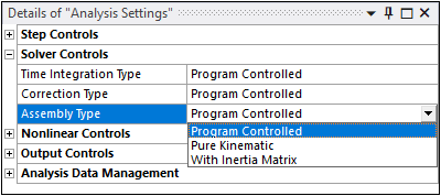
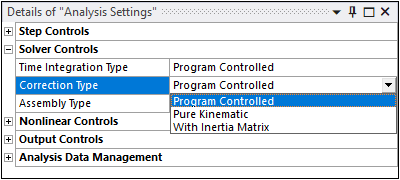
The Details view Solver Controls options for the Time Integration Type include:
Time Integration Type field. Available time integration algorithms include:
Program Controlled (default setting): The application selects the most appropriate method based on the current model. If the model contains only rigid bodies, 4th order Runge-Kutta is used. If the model contains flexible bodies (Condensed Parts), the Stabilized Generalized Alpha option is selected automatically.
Runge-Kutta 4: Fourth Order Runge-Kutta.
Implicit Generalized Alpha: Implicit time integration based on the Generalized-α method.
Stabilized Generalized Alpha: Implicit time integration based on the Stabilized Generalized-α method.
MJ Time Stepping: Moreau-Jean time-stepping integration.
Correction Type: (default), , or .
Assembly Type: (default), , or .