


Physical deformations can be calculated on and inside a part or an assembly. Fixed supports prevent deformation: locations without a fixed support usually experience deformation relative to the original location. Deformations are calculated relative to the part or assembly world coordinate system.
 Component deformations (Directional
Deformation)
Component deformations (Directional
Deformation)
 Deformed shape (Total Deformation vector)
The three component deformations Ux, Uy, and Uz, and the deformed shape U are available as individual results.
Scoping is also possible to both geometric entities and to underlying meshing entities (see example below). Numerical data is for deformation in the global X, Y, and Z directions. These results can be viewed with the model under wireframe display, facilitating their visibility at interior nodes.
Go to a section topic:
Limitation
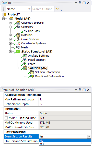
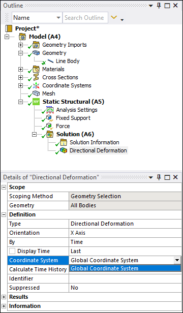
Limitation: The application currently has a limitation. If you have a Line Body model and the Model Type property is set to either or (elements), and the Beam Section Results property of the Solution object is set to , the application does not display result contours in the Solution Coordinate System. This is true even if you set the Coordinate System property of a result object to . The contours will display in the .
|
|
|
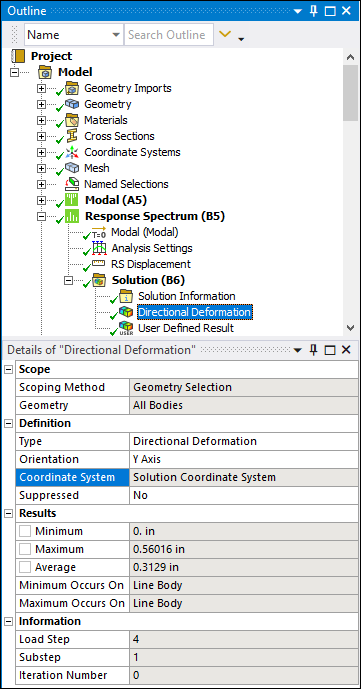
This limitation is also applicable if you are performing a Response Spectrum analysis where the Coordinate System property is read-only and set to . Result contours display in the . In this scenario, you can display the contours in the by setting the Beam Section Results property to .
Scoping Deformation Results to Mesh Nodes
The following example illustrates how to obtain deformation results for individual nodes in a model. The nodes are specified using criteria based named selections.
Create a named selection by highlighting the Model object and select the option from the Insert group of the Model Context tab.
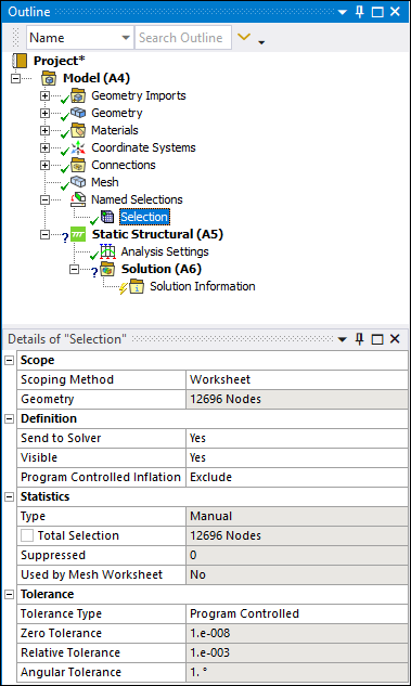
Highlight the Selection object and in the Details, set the Scoping Method property to Worksheet.
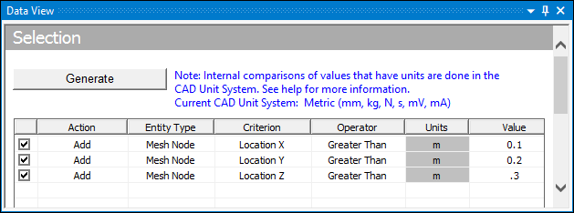
In the Worksheet, add a row and specify the following. Refer to Specifying Named Selections using Worksheet Criteria for assistance, if needed.
Entity Type = Mesh Node.
Criterion = Location X.
Operator = Greater Than.
Value = 0.1.
Add a second row with Criterion = Location Y, Value = 0.2, and all remaining items set the same as the first row.
Add a third row with Criterion = Location Z, Value = 0.3, and all remaining items set the same as the first row. The table should appear as follows:
Click the button. The Geometry property displays the number of nodes that meet the criteria defined in the Worksheet.
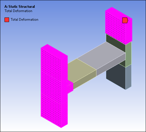
After applying loads and supports to the model, add a Total Deformation result object, highlight the object, set Scoping Method to Named Selection, and set Named Selection to the Selection object defined above that includes the mesh node criteria. Before solving, annotations are displayed at each selected node as shown below.
Solve the analysis. Any element containing a selected node will display a contour color at the node. If all nodes on the element are selected, the element will display contour colors on all facets. Element facets that contain unselected nodes will be transparent. An example is shown below.
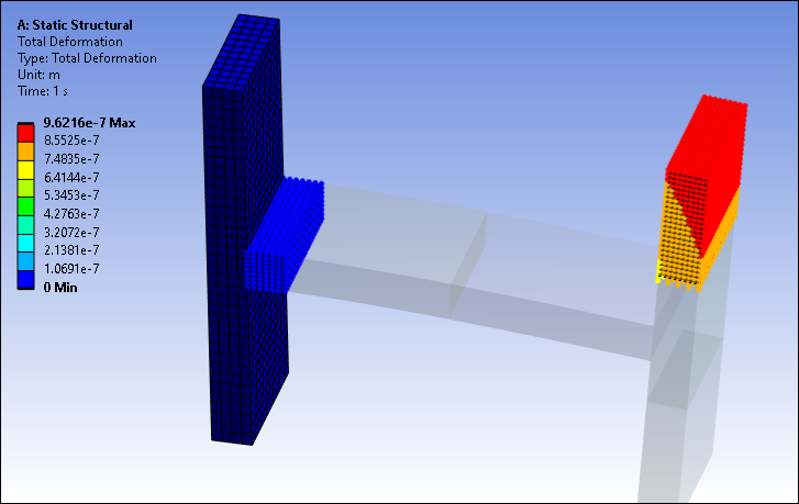
Note that all element facets are drawn, not just the facets on the surface or skin of the model.
To possibly reduce clutter for complex models, the size of the dots representing the nodes can be changed by selecting the option from the Display group of Result Context Tab.
Working with Deformations
Deformations can be used to:
Set Alert objects.
Control accuracy and convergence and to view converged results.
Study deformations in a selected or scoped area of a part or an assembly.
Important: The deformation result can exhibit a node-based display limitation. If a node represents a remote point, the application does not process result data for it and as a result, Mechanical does not display result data. Deformed shapes, deformation contour colors, and deformation MIN/MAX values can differ from the displays (and listings) of Mechanical APDL commands, such as PRNSOL, PLNSOL, and MONITOR.
Velocity and Acceleration Deformations
In addition to deformation results, velocity and acceleration results are also available for Transient Structural, Harmonic Response (Full and MSUP), Rigid Dynamics, Random Vibration, and Response Spectrum analyses. Both total and directional components are available for the Transient Structural and Harmonic Response analyses but only directional components are available for Random Vibration and Response Spectrum ( is not available).
Considerations for Random Vibration Analyses
For Random Vibration analyses, only component directional deformations are available because the directional results from the solver are statistical in nature. The X, Y, and Z displacements cannot be combined to get the magnitude of the total displacement. The same holds true for other derived quantities such as principal stresses.
Directional Deformation, Directional Velocity, and Directional Acceleration result objects in Random Vibration analyses also include the following additional items in the Details:
Reference - Read-only reference indication that depends on the directional result. Possible indications are:
Relative to base motion for a Directional Deformation result.
Absolute (including base motion) for a Directional Velocity or Directional Acceleration result.
Scale Factor - A multiple of standard deviation values (with zero mean value) that you can enter which determines the probability of the time the response will be less than the standard deviation value. By default, the results output by the solver are 1 Sigma, or one standard deviation value. You can set the Scale Factor to 2 Sigma, 3 Sigma, or to User Input, in which case you can enter a custom scale factor in the Scale Factor Value field.
Probability - Read-only indication of the percentage of the time the response will be less than the standard deviation value as determined by your entry in the Scale Factor field. A Scale Factor of 1 Sigma = a Probability of 68.3 %. 2 Sigma = 95.951 %. 3 Sigma = 99.737 %.