


Background
An Eigenvalue Buckling analysis predicts the theoretical buckling strength of an ideal elastic structure. This method corresponds to the textbook approach to an elastic buckling analysis: for instance, an eigenvalue buckling analysis of a column matches the classical Euler solution. However, imperfections and nonlinearities prevent most real-world structures from achieving their theoretical elastic buckling strength. Therefore, an Eigenvalue Buckling analysis often yields quick but non-conservative results.
A more accurate approach to predicting instability is to perform a nonlinear buckling analysis. This involves a static structural analysis with large deflection effects turned on. A gradually increasing load is applied in this analysis to seek the load level at which your structure becomes unstable. Using the nonlinear technique, your model can include features such as initial imperfections, plastic behavior, gaps, and large-deflection response. In addition, using deflection-controlled loading, you can even track the post-buckled performance of your structure (which can be useful in cases where the structure buckles into a stable configuration, such as "snap-through" buckling of a shallow dome, as illustrated below).

(a) Nonlinear load-deflection curve, (b) Eigenvalue buckling curve.
Eigenvalue Buckling in Mechanical
In Mechanical, an Eigenvalue Buckling analysis is a linear analysis and therefore cannot account for nonlinearities. It employs the Linear Perturbation Analysis procedure of Mechanical APDL. This procedure requires a pre-loaded environment from which it draws solution data for use in the Eigenvalue Buckling analysis. Based on this requirement, an Eigenvalue Buckling analysis can consider nonlinearities that are present in the pre-stressed environment allowing you to attain a more accurate real-world solution as compared to a traditional linear preloaded state.
Note: The application supports the use of the Samcef solver for this analysis type. However, the information presented below applies to the use of the Mechanical APDL Solver only.
Points to Remember
An Eigenvalue Buckling analysis must be linked to (proceeded by) a Static Structural Analysis. This static analysis can be either linear or nonlinear and the linear perturbation procedure refers to it as the "base analysis" (as either linear or nonlinear).
The nonlinearities present in the static analysis can be the result of nonlinear:
Geometry (the Large Deformation property is set to )
Contact status ( A contact condition with the Type property set to anything other than or is treated as a non-linearity for contact. In addition, when the Small Sliding property set to , the system is treated as non-linear contact.)
Material (such as the definition of nonlinear material properties in Engineering Data, hyperelasticity, plasticity, etc.)
Connection (such as nonlinear joints and nonlinear springs)
A structure can have an infinite number of buckling load factors. Each load factor is associated with a different instability pattern. Typically the lowest load factor is of interest.
Based upon how you apply loads to a structure, load factors can either be positive or negative. The application sorts load factors from the most negative values to the most positive values. The minimum buckling load factor may correspond to the smallest eigenvalue in absolute value.
For Pressure boundary conditions in the Static Structural analysis: if you define the load with the option for faces (3D) or edges (2-D), you could experience an additional stiffness contribution called the "pressure load stiffness" effect. The option causes the pressure to act as a follower load, which means that it continues to act in a direction normal to the scoped entity even as the structure deforms. Pressure loads defined with the or options act in a constant direction even as the structure deforms. For a given pressure value in the upstream static system, the option and the / options can produce significantly different buckling load factors in the follow-on Eigenvalue Buckling analysis.
Buckling mode shapes do not represent actual displacements but help you to visualize how a part or an assembly deforms when buckling.
The procedure that the Mechanical APDL solver uses to evaluate buckling load factors is dependent upon whether the pre-stressed Eigenvalue Buckling analysis is linear-based (linear prestress analysis) or nonlinear-based (nonlinear prestress analysis), as described below.
- Linear-based Eigenvalue Buckling Analysis
Note the following for an Eigenvalue Buckling analysis when the base analysis is linear:
You can only define loading conditions in the upstream analysis.
The results calculated by the Eigenvalue Buckling analysis are buckling load factors that scale all of the loads applied in the upstream Static Structural analysis. For example, if you applied a 10 N compressive load on a structure in the static analysis and if the Eigenvalue Buckling analysis calculates a load factor of 1500, then the predicted buckling load is 1500x10 = 15000 N. Because of this, it is typical to apply unit loads in the static analysis that precedes the buckling analysis.
The solver applies the buckling load factor to all the loads specified in the upstream static analysis.
Note that the load factors represent scaling factors for all loads. If certain loads are constant (self-weight gravity loads) while other loads are variable (externally applied loads), you need to take special steps to ensure accurate results. For example, you can iterate on the Eigenvalue buckling solution, adjusting the variable loads until the load factor becomes 1.0 (or nearly 1.0, within some convergence tolerance). Consider the example below: a pole has a self-weight W0 that supports an externally-applied load, A. To determine the limiting value of A in an Eigenvalue Buckling analysis, you could solve repetitively, using different values for A, until you find a load factor acceptably close to 1.0.
If you receive all negative buckling load factor values for your Eigenvalue Buckling analysis and you wish to see them in the positive values, or vice versa, reverse the direction of all of the loads you applied in Static Structural analysis.
You can apply a nonzero constraint in the Static Structural analysis. The load factors calculated in the buckling analysis should also be applied to these nonzero constraint values. However, the buckling mode shape associated with this load will show the constraint to have zero value.
- Nonlinear-based Eigenvalue Buckling Analysis
Note the following for an Eigenvalue Buckling analysis when the base analysis is nonlinear:
At least one form of nonlinearity must be defined in the upstream static analysis.
You must define at least one load in the buckling analysis to proceed with the solution. To enable this, set the Keep Pre-Stress Load-Pattern property to (default). This retains the loading pattern from the Static Structural analysis in the Eigenvalue Buckling analysis. Setting the property to requires you to define a new loading pattern for the Eigenvalue Buckling analysis. This new loading pattern can be completely different from that of the prestress analysis.
In a nonlinear-based Eigenvalue Buckling analysis, load multipliers scale the loads applied in buckling analysis ONLY. When estimating the ultimate buckling load for the structure, you must account for the loading applied in both analyses. The equation to calculate the ultimate buckling load for the nonlinear-based Eigenvalue Buckling analysis is:
FBUCKLING = FRESTART + λi · FPERTRUB
where:
FBUCKLING = The ultimate buckling load for the structure.
FRESTART = Total loads in Static Structural analysis at the specified restart load step.
λi = Buckling load factor for the "i'th" mode.
FPERTRUB = Perturbation loads applied in buckling analysis.
For example, if you applied a 100 N compressive force on a structure in the static analysis and a compressive force of 10 N in the Eigenvalue Buckling analysis and you get a load factor of 15, then the ultimate buckling load for the structure is 100 + (15 x 10) = 250 N.
You can verify the ultimate buckling load of the above equation using the buckling of a one dimensional column. However, calculating the ultimate buckling load for 2D and 3D problems with different combinations of loads applied in the Static Structural and Eigenvalue Buckling analyses may not be as straightforward as the 1D column example. This is because the FRESTART and FPERTRUB values are essentially the effective loading values in the static and buckling analyses, respectively.
For example, consider a cantilever beam that has a theoretical ultimate buckling strength of 1000N and that is subjected to a compressive force (A) of 250N. The procedure to calculate the ultimate buckling load (F), based on the load factors evaluated by Mechanical for linear-based and nonlinear-based Eigenvalue Buckling analyses is illustrated in the following schematic.
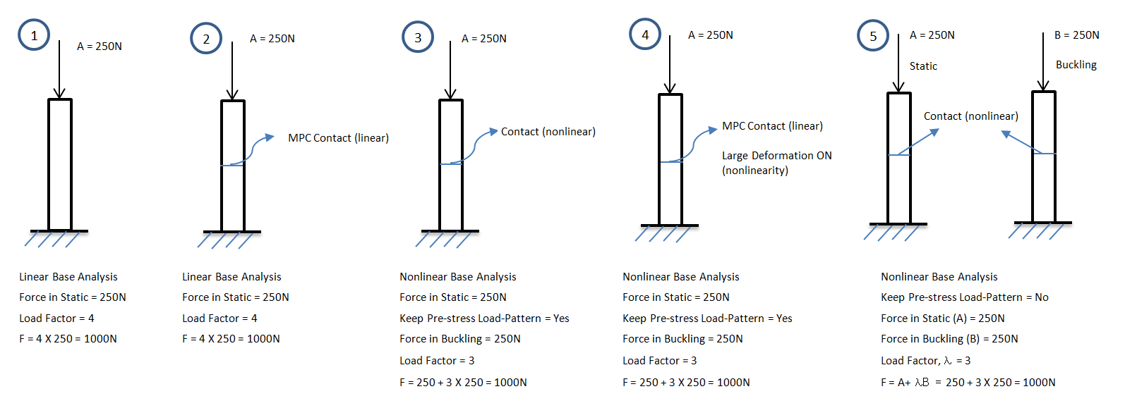
Note: As illustrated, cases (3) and (5) are identical as the base analysis is nonlinear because of nonlinear contact definition. In Case (3), setting the Keep Pre-Stress Load-Pattern property to automatically retains the loading from the pre-stress analysis. As a result, there is no need to define new loads for the buckling analysis in Case 3. For Case 5, the Keep Pre-Stress Load-Pattern property is set to , enabling you to define a new load pattern in the buckling analysis that can be completely different from that of the Static Structural analysis.
The buckling load factor evaluated in nonlinear-based Eigenvalue Buckling should be applied to all of the loads used in the buckling analysis.
If you receive all negative buckling load factor values for your Eigenvalue Buckling analysis and you wish to see them in the positive values, or vice versa, reverse the direction of all of the loads you applied in the Static Structural analysis when the Keep Pre-Stress Load-Pattern property is set to . If this property is set to , reverse the direction of all of the loads that you applied in Eigenvalue Buckling analysis.
Preparing the Analysis
Create Analysis System
 Basic general information about this topic
 ... for this analysis type:
Because this analysis is based on the Static Structural solution, a Static Structural analysis is a prerequisite. This linked setup allows the two analysis systems to share resources such as engineering data, geometry, and boundary condition type definitions.
From the Toolbox, drag a Static Structural template to the Project Schematic. Then, drag an Eigenvalue Buckling template directly onto the Solution cell of the Static Structural template. The proper linking is illustrated below.

Define Engineering Data
Basic general information about this topic
... for this analysis type:
Young's modulus (or stiffness in some form) must be defined.
Material properties can be linear, nonlinear, isotropic or orthotropic, and constant or temperature-dependent.
Attach Geometry
Basic general information about this topic
... for this analysis type:
There are no specific considerations for an Eigenvalue Buckling analysis.
Define Part Behavior
Basic general information about this topic
... for this analysis type:
There are no specific considerations for an Eigenvalue Buckling analysis.
Define Connections
Basic general information about this topic
... for this analysis type:
- Linear-based Eigenvalue Buckling Analysis
The following contact settings are considered linear contact behaviors for Eigenvalue Buckling analyses. If any other contact settings are used, the analysis will be considered a Nonlinear-based Eigenvalue Buckling analysis.
The Formulation property is set to or .
Or...
The Type property is set to or and is active.
Springs with linear stiffness definition are taken into account if they are present in the static analysis.
Only Bushing and General joints enable you to solve an analysis with nonlinear Joint Stiffness. Mechanical considers all other joint types to be linear. The application accounts for linear joints if they are present in the static analysis.
- Nonlinear-based Eigenvalue Buckling Analysis
All nonlinear connections (including nonlinear springs and joints) are allowed. Any contact options other than the ones mentioned above would trigger a nonlinear-based Eigenvalue Buckling analysis.
Apply Mesh Controls/Preview Mesh
Basic general information about this topic
... for this analysis type:
There are no considerations specifically for an Eigenvalue Buckling analysis.
Establish Analysis Settings
Basic general information about this topic
... for this analysis type:
For an Eigenvalue Buckling analysis, the basic Analysis Settings include:
- Options
Use the Max Modes to Find property to specify the number of buckling load factors and corresponding buckling mode shapes of interest. Typically the first (lowest) buckling load factor is of interest. The default value for this field is
2. You can change this default setting under the Buckling category of the Frequency options in the Options preference dialog.The Keep Pre-Stress Load-Pattern property is available for nonlinear-based Eigenvalue Buckling analyses. Use this property to specify whether you want to retain the pre-stress loading pattern to generate the perturbation loads in the Eigenvalue Buckling analysis. The default setting for this property is , which automatically retains the structural loading pattern for the buckling analysis (refer to the ALLKEEPLoadControl key setting for PERTURB command). Setting the property to requires you to define a new loading pattern for the Eigenvalue Buckling analysis (refer to PARKEEPLoadControl key setting for PERTURB command).
Important: Because the PARKEEPLoadControl key retains all displacements applied in Static Structural analysis for reuse in Eigenvalue Buckling analysis, any non-zero displacements applied in static analysis act as loads in Eigenvalue Buckling analysis. If you specifying different load types in the buckling analysis that are scoped to the same geometric entities and in the same direction, may be ignored. Define your new loading pattern carefully.
- Solver Controls
Solver Type: The default option, , enables the application to select the appropriate solver type. Options include , , and . By default, the option uses the solver for linear-based Eigenvalue Buckling analyses and solver for nonlinear-based Eigenvalue Buckling analyses.
Note: Both the and solvers evaluate the buckling solutions for most engineering problems. If you experience a solution failure using one of the solvers because it cannot find the requested modes, it may help to switch the solvers. If both of the solvers fail to find the solution, then review your model carefully for possible stringent input specifications or loading conditions.
Include Negative Load Multiplier: The default option and the option extract both the negative and positive eigenvalues (load multipliers). The option only extracts positive eigenvalues (load multipliers).
- Output Controls
By default, only buckling load factors and corresponding buckling mode shapes are calculated. You can request Stress and Strain results to be calculated but note that "stress" results only show the relative distribution of stress in the structure and are not real stress values.
Note: The Output Controls category is only exposed for the Mechanical APDL solver.
- Analysis Data Management
The properties of this category enable you to define whether or not to automatically save the Mechanical APDL database as well as automatically delete unneeded files.
Define Initial Conditions
Basic general information about this topic
... for this analysis type:
You must specify a Static Structural analysis that is using the same model in the initial condition environment, and:
Because an Eigenvalue Buckling analysis must be preceded by a Static Structural analysis, you need to specify the same solver type for each, either Mechanical APDL or Samcef.
The Pre-Stress Environment property in the Pre-Stress (Static Structural) initial condition object displays whether the pre-stress environment is considered linear or nonlinear for the Eigenvalue Buckling analysis.
If the Static Structural analysis has multiple result sets, the value from any restart point available in the Static Structural analysis can be used as the basis for the Eigenvalue Buckling analysis. See the Restarts from Multiple Result Sets topic in the Applying Pre-Stress Effects Help section for more information.
Basic general information about this topic
... for this analysis type:
Loads are supported by Eigenvalue Buckling analysis only when the pre-stressed environment has nonlinearities defined.
The following loads are supported for a nonlinear-based Eigenvalue Buckling analysis:
Direct FE (node-based Named Selection scoping and constant loading only):
Note:
Choosing to keep the default setting () for the Keep Pre-Stress Load-Pattern property retains the pre-stress loading pattern for the buckling analysis and no additional load definition is necessary.
For , the only definition option is . This results in the "pressure load stiffness" effect. To avoid the pressure stiffness effect, apply an equivalent load to the same surface and set the Divide Load by Nodes property to . The equivalent force is equal to the value of the pressure multiplied by the area of the scoped surface.
The node-based Named Selections used with the above Direct FE Loads cannot contain nodes scoped to a rigid body.
No loading conditions can be created in a linear-based Eigenvalue Buckling analysis. The supports as well as the stress state from the linked Static Structural analysis are used in the linear-based Eigenvalue Buckling analysis. See the Apply Pre-Stress Effects for Implicit Analysis section for more information about using a pre-stressed environment.
Solve
Basic general information about this topic
... for this analysis type:
Solution Information continuously updates any listing output from the solver and provides valuable information on the behavior of the structure during the analysis.
Review Results
Basic general information about this topic
... for this analysis type:
You can view the buckling mode shape associated with a particular load factor by displaying a contour plot or by animating the deformed mode shape. The contours represent relative displacement of the part.
Buckling mode shape displays are helpful in understanding how a part or an assembly deforms when buckling, but do not represent actual displacements.
"Stresses" from an Eigenvalue Buckling analysis do not represent actual stresses in the structure, but they give you an idea of the relative stress distributions for each mode. You can make Stress and Strain results available in the buckling analysis by setting the proper Output Controls before the solution is processed.