


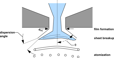
Another important type of atomizer is the pressure-swirl atomizer, sometimes referred to by the gas-turbine community as a simplex atomizer. This type of atomizer accelerates the liquid through nozzles known as swirl ports into a central swirl chamber. The swirling liquid pushes against the walls of the swirl chamber and develops a hollow air core. It then emerges from the orifice as a thinning sheet, which is unstable, breaking up into ligaments and droplets. The pressure-swirl atomizer is very widely used for liquid-fuel combustion in gas turbines, oil furnaces, and direct-injection spark-ignited automobile engines. The transition from internal injector flow to fully-developed spray can be divided into three steps: film formation, sheet breakup, and atomization. A sketch of how this process is thought to occur is shown in Figure 12.21: Theoretical Progression from the Internal Atomizer Flow to the External Spray.
The interaction between the air and the sheet is not well understood. It is generally accepted that an aerodynamic instability causes the sheet to break up. The mathematical analysis below assumes that Kelvin-Helmholtz waves grow on the sheet and eventually break the liquid into ligaments. It is then assumed that the ligaments break up into droplets due to varicose instability. Once the liquid droplets are formed, the spray evolution is determined by drag, collision, coalescence, and secondary breakup.
The pressure-swirl atomizer model used in Ansys Fluent is called the Linearized Instability Sheet Atomization (LISA) model of Schmidt et al. [583]. The LISA model is divided into two stages:
film formation
sheet breakup and atomization
Both parts of the model are described below.
The centrifugal motion of the liquid within the injector creates
an air core surrounded by a liquid film. The thickness of the film
at the injector exit,  , is related to the mass flow rate by:
 | (12–375) |
where  is
the injector exit diameter, and
is
the injector exit diameter, and  is the effective mass flow rate, which
is defined by Equation 12–357. The other unknown
in Equation 12–375 is
is the effective mass flow rate, which
is defined by Equation 12–357. The other unknown
in Equation 12–375 is  , the axial component of velocity
at the injector exit. This quantity depends on internal details of
the injector and is difficult to calculate from first principles.
Instead, the approach of Han et al. [230] is used.
The total velocity is assumed to be related to the injector pressure
by
, the axial component of velocity
at the injector exit. This quantity depends on internal details of
the injector and is difficult to calculate from first principles.
Instead, the approach of Han et al. [230] is used.
The total velocity is assumed to be related to the injector pressure
by
 | (12–376) |
where  is the velocity
coefficient. Lefebvre [351] has noted that
is the velocity
coefficient. Lefebvre [351] has noted that  is a function of the injector design and
injection pressure. If the swirl ports are treated as nozzles and
if it is assumed that the dominant portion of the pressure drop occurs
at those ports,
is a function of the injector design and
injection pressure. If the swirl ports are treated as nozzles and
if it is assumed that the dominant portion of the pressure drop occurs
at those ports,  is the expression
for the discharge coefficient (
is the expression
for the discharge coefficient ( ). For single-phase nozzles
with sharp inlet corners and
). For single-phase nozzles
with sharp inlet corners and  ratios of 4, a typical
  value is 0.78
or less [370]. If the nozzles are cavitating,
the value of
value is 0.78
or less [370]. If the nozzles are cavitating,
the value of  may be as low as 0.61. Hence,
0.78 could be considered a practical upper bound for
may be as low as 0.61. Hence,
0.78 could be considered a practical upper bound for  . The effect of other momentum losses is
approximated by reducing
. The effect of other momentum losses is
approximated by reducing  by 10% to
0.7.
by 10% to
0.7.
Physical limits on  require that
it be less than unity from conservation of energy, yet be large enough
to permit sufficient mass flow. The requirement that the size of the
air-core be non-negative implies the following constraint on the film
thickness,
require that
it be less than unity from conservation of energy, yet be large enough
to permit sufficient mass flow. The requirement that the size of the
air-core be non-negative implies the following constraint on the film
thickness,  :
:
 | (12–377) |
Combining this with Equation 12–375 gives
the following constraint on the axial velocity,  :
:
 | (12–378) |
This can be combined with Equation 12–376 and  , where
  is the spray half-angle
and is assumed to be known. This yields a constraint on
is the spray half-angle
and is assumed to be known. This yields a constraint on  :
:
 | (12–379) |
Thus, Fluent uses the following expression for  :
:
 | (12–380) |
Assuming that  is known, Equation 12–376 can be used to find
  . Once
  is determined,
  is found from
 | (12–381) |
At this point, the thickness and axial component of the liquid
film are known at the injector exit. The tangential component of velocity
( ) is assumed to be equal to the radial velocity
component of the liquid sheet downstream of the nozzle exit. The axial
component of velocity is assumed to remain constant.
) is assumed to be equal to the radial velocity
component of the liquid sheet downstream of the nozzle exit. The axial
component of velocity is assumed to remain constant.
The pressure-swirl atomizer model includes the effects of the surrounding gas, liquid viscosity, and surface tension on the breakup of the liquid sheet. Details of the theoretical development of the model are given in Senecal et al. [587] and are only briefly presented here. For a more robust implementation, the gas-phase velocity is neglected in calculating the relative liquid-gas velocity and is instead set by you. This avoids having the injector parameters depend too heavily on the usually under-resolved gas-phase velocity field very near the injection location.
The model assumes that a two-dimensional, viscous, incompressible
liquid sheet of thickness  moves with velocity
  through a quiescent, inviscid,
incompressible gas medium. The liquid and gas have densities of
through a quiescent, inviscid,
incompressible gas medium. The liquid and gas have densities of  and
and  ,
respectively, and the viscosity of the liquid is
,
respectively, and the viscosity of the liquid is  .
A coordinate system is used that moves with the sheet, and a spectrum
of infinitesimal wavy disturbances of the form
.
A coordinate system is used that moves with the sheet, and a spectrum
of infinitesimal wavy disturbances of the form
 | (12–382) |
is imposed on the initially steady motion. The spectrum of disturbances
results in fluctuating velocities and pressures for both the liquid
and the gas. In Equation 12–382,  is the initial wave amplitude,
  is
the wave number, and
is
the wave number, and  is the complex growth rate. The most unstable disturbance
has the largest value of
is the complex growth rate. The most unstable disturbance
has the largest value of  , denoted here by
  , and is assumed to
be responsible for sheet breakup. Thus, it is desired to obtain a
dispersion relation
, and is assumed to
be responsible for sheet breakup. Thus, it is desired to obtain a
dispersion relation  from which
the most unstable disturbance can be calculated as a function of wave
number.
from which
the most unstable disturbance can be calculated as a function of wave
number.
Squire [628], Li and Tankin [365], and Hagerty and Shea [225] have
shown that two solutions, or modes, exist that satisfy the governing
equations subject to the boundary conditions at the upper and lower
interfaces. The first solution, called the sinuous mode, has waves
at the upper and lower interfaces in phase. The second solution is
called the varicose mode, which has the waves at the upper and lower
interfaces  radians out of phase. It has been shown
by numerous authors (for example, Senecal et al. [587]) that the sinuous mode dominates the growth of
varicose waves for low velocities and low gas-to-liquid density ratios.
In addition, it can be shown that the sinuous and varicose modes become
indistinguishable for high-velocity flows. As a result, the atomization
model in Ansys Fluent is based upon the growth of sinuous waves on the
liquid sheet.
radians out of phase. It has been shown
by numerous authors (for example, Senecal et al. [587]) that the sinuous mode dominates the growth of
varicose waves for low velocities and low gas-to-liquid density ratios.
In addition, it can be shown that the sinuous and varicose modes become
indistinguishable for high-velocity flows. As a result, the atomization
model in Ansys Fluent is based upon the growth of sinuous waves on the
liquid sheet.
As derived in Senecal et al. [587], the dispersion relation for the sinuous mode is given by
 | (12–383) |
 | (12–384) |
where  and
and  .
.
Above a critical Weber number of  =
27/16 (based on the liquid velocity, gas density, and sheet half-thickness),
the fastest-growing waves are short. For
=
27/16 (based on the liquid velocity, gas density, and sheet half-thickness),
the fastest-growing waves are short. For  , the wavelengths are long compared to the
sheet thickness. The speed of modern high pressure fuel injection
systems is high enough to ensure that the film Weber number is well
above this critical limit.
, the wavelengths are long compared to the
sheet thickness. The speed of modern high pressure fuel injection
systems is high enough to ensure that the film Weber number is well
above this critical limit.
An order-of-magnitude analysis using typical values shows that the terms of second order in viscosity can be neglected in comparison to the other terms in Equation 12–384. Using this assumption, Equation 12–384 reduces to
 | (12–385) |
 | (12–386) |
For waves that are long compared with the sheet thickness, a
mechanism of sheet disintegration proposed by Dombrowski and Johns [145] is adopted. For long waves, ligaments are
assumed to form from the sheet breakup process once the unstable waves
reach a critical amplitude. If the surface disturbance has reached
a value of  at breakup, a breakup
time,
at breakup, a breakup
time,  , can be evaluated:
 | (12–387) |
where  , the maximum growth rate, is found by numerically
maximizing Equation 12–386 as a function of
, the maximum growth rate, is found by numerically
maximizing Equation 12–386 as a function of  . The maximum is found using
a binary search that checks the sign of the derivative. The sheet
breaks up and ligaments will be formed at a length given by
. The maximum is found using
a binary search that checks the sign of the derivative. The sheet
breaks up and ligaments will be formed at a length given by
 | (12–388) |
where the quantity  is an empirical sheet constant that you must specify. The
default value of 12 was obtained theoretically by Weber [695] for liquid
jets. Dombrowski and Hooper [144] showed that a value of 12 for the
sheet constant agreed favorably with experimental sheet breakup lengths over a range of Weber
numbers from 2 to 200.
is an empirical sheet constant that you must specify. The
default value of 12 was obtained theoretically by Weber [695] for liquid
jets. Dombrowski and Hooper [144] showed that a value of 12 for the
sheet constant agreed favorably with experimental sheet breakup lengths over a range of Weber
numbers from 2 to 200.
The diameter of the ligaments formed at the point of breakup can be obtained from a mass balance. If it is assumed that the ligaments are formed from tears in the sheet twice per wavelength, the resulting diameter is given by
 | (12–389) |
where  is the wave number corresponding
to the maximum growth rate,
is the wave number corresponding
to the maximum growth rate,  . The ligament diameter depends on the sheet
thickness, which is a function of the breakup length. The film thickness
is calculated from the breakup length and the radial distance from
the center line to the mid-line of the sheet at the atomizer exit,
. The ligament diameter depends on the sheet
thickness, which is a function of the breakup length. The film thickness
is calculated from the breakup length and the radial distance from
the center line to the mid-line of the sheet at the atomizer exit,
 :
:
 | (12–390) |
This mechanism is not used for waves that are short compared to the sheet thickness. For short waves, the ligament diameter is assumed to be linearly proportional to the wavelength that breaks up the sheet,
 | (12–391) |
where  , or the ligament constant,
is equal to 0.5 by default.
, or the ligament constant,
is equal to 0.5 by default.
In either the long-wave or the short-wave case, the breakup from ligaments to droplets is assumed to behave according to Weber’s [695] analysis for capillary instability.
 | (12–392) |
Here,  is the Ohnesorge number, which
is a combination of the Reynolds number and the Weber number (see Jet Stability Analysis for more details about Oh). Once
is the Ohnesorge number, which
is a combination of the Reynolds number and the Weber number (see Jet Stability Analysis for more details about Oh). Once  has been determined from Equation 12–392, it is assumed that this droplet diameter
is the most probable droplet size of a Rosin-Rammler distribution
with a spread parameter of 3.5 and a default dispersion angle of 6° (which can be modified in the user interface).
The choice of spread parameter and dispersion angle is based on past
modeling experience [582]. It is important
to note that the spray cone angle must be specified by you when using
this model.
has been determined from Equation 12–392, it is assumed that this droplet diameter
is the most probable droplet size of a Rosin-Rammler distribution
with a spread parameter of 3.5 and a default dispersion angle of 6° (which can be modified in the user interface).
The choice of spread parameter and dispersion angle is based on past
modeling experience [582]. It is important
to note that the spray cone angle must be specified by you when using
this model.