
What's New in Mechanical
|
Geometry
External Model
|
LS-DYNA System
Analysis
Acoustics Analyses
Coupled Field Analyses
Structural Optimization
|
Loads/Supports/Conditions
Solution
Results and Post Processing
|
Graphics
Accelerated Graphics/Animation
In order to display more accurate lighting for results with extremely large deformations, the Options dialog, Graphics group, preference, Use Faceted Lighting for Accelerated Graphics/Animation, is now active (set to Yes) by default. The concession for this setting is that models, typically those with low resolution meshes, may produce a slightly more faceted display.
New Linux Capabilities
The following graphical features are now supported on the Linux platform:
Accelerated Graphics Feature
Accelerated Animation Feature
Anti-Aliasing (MSAA) Preference
Display Graph Option
Probe Tool and Hit Point Coordinate Preference
Text Display Enhancements
The quality of the text displayed in the Geometry window has been improved this release.
Geometry
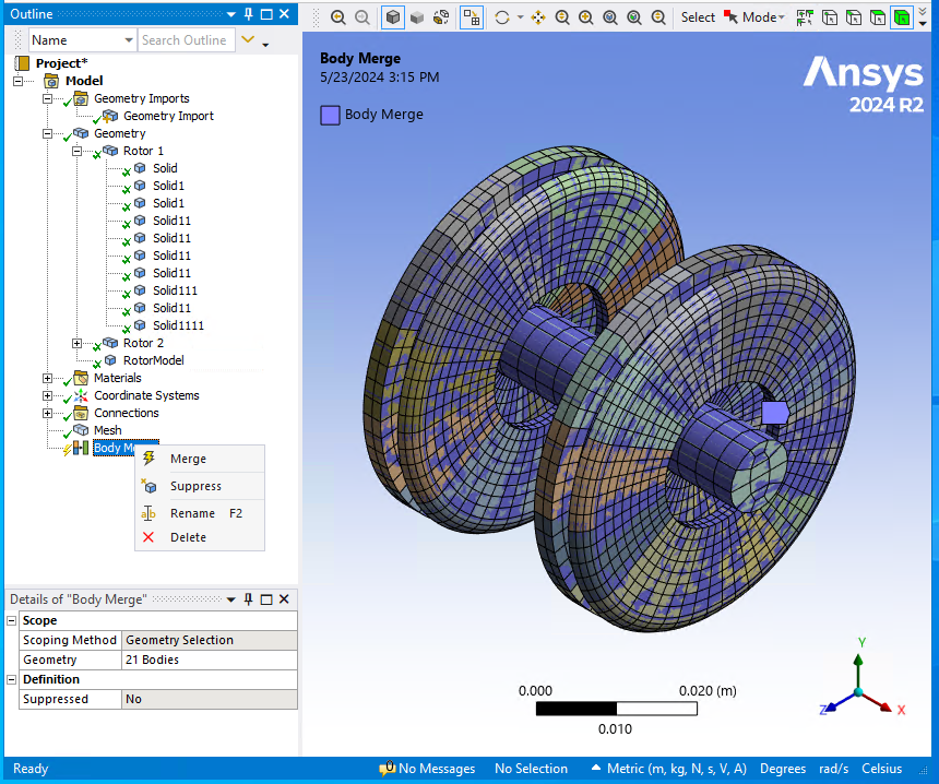
Body Merge
The new Body Merge feature enables you to combine multiple solid bodies with shared faces into a single body. The mesh is also merged if the model has been meshed. This simplifies complicated geometries by reducing the number of bodies in a model, which is especially useful for complex parts. Body Merge can also be used to merge bodies that were previously sliced to generate a hex dominant mesh.

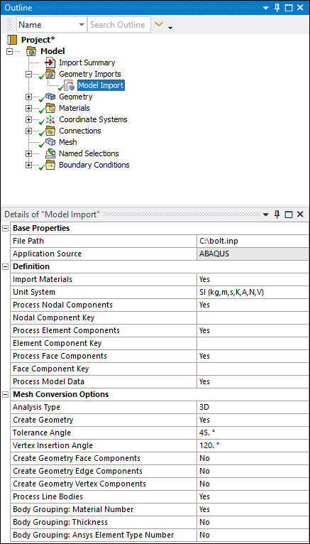
Importing External Mesh Files
Now, when you open Mechanical independently (only), you can import LS-DYNA Input (.k and .key), or Abaqus (.inp) files directly into the application using the Add Model Import option available from the Geometry Imports object.
External Model
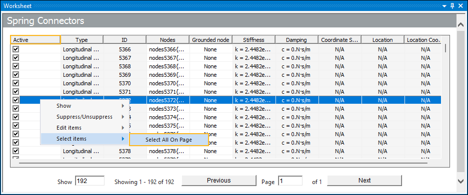
Worksheet Enhancements for Imported Mesh Data
Several changes have been made to the worksheet that presents data for imported mesh data:
The Check/Uncheck column of the worksheet has been renamed Active to represent the function of the column more clearly. That is, activating and/or deactivating the data of a worksheet row.
You can also now select multiple worksheets row and select the Active check box of any one of the rows to change the status of all of the rows.
A new context (right-click) menu option, Select Items > Select All On Page, enables you to automatically select all rows in the currently displayed page of the worksheet.
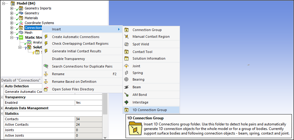
Connections
Connections Manager
Connections Manager is a new extension that provides capabilities, through the 1D Connection Group object, to automatically generate and manage connection objects for an entire model or a group of bodies within a model.
Rigid-To-Flexible Contact
The application no longer creates a duplicate layer of target elements (called an insulation layer) for contact regions defined between a rigid body surface and a flexible body. This optimization significantly improves solution processing performance for large assembly models.
Cylindrical Smoothing
When you set the Contact Geometry Correction or Target Geometry Correction properties to Smoothing and the Orientation property to Program Controlled, you can now select multiple cylindrical faces for the scoping of the Contact Region.
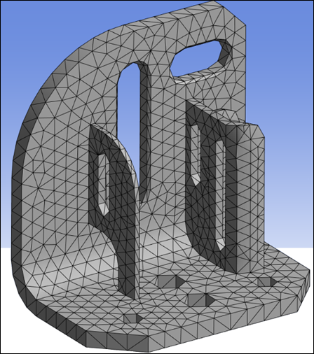
Mesh
Geometry Fidelity
The Geometry Fidelity feature ensures the nodes of the mesh lie on the scoped geometry faces, including midside nodes for quadratic elements. This can be important in areas of the model where contact will be used.
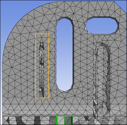
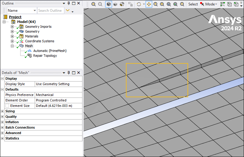
Automatic (PrimeMesh)
The Automatic (PrimeMesh) Method for fast and high quality shell meshing has been enhanced to:
Provide an Auto Repair Topology feature to automatically repair topologies of the scoped bodies in order to defeature thin or sharp faces.
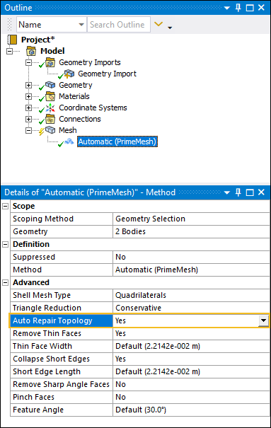
Include a Feature Angle property for the Method (shown above) as well as the Repair Topology Control object, so you can specify the minimum angle at which the application repairs geometry features.
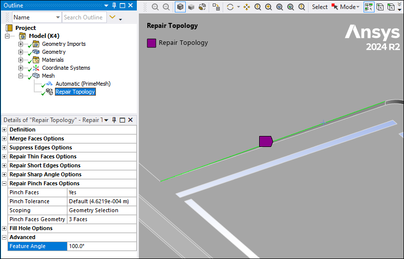
Set to 30 degrees by default to avoid the loss of feature edges, you can now increase the angle to perform more aggressive defeaturing and enable higher quality mesh generation.
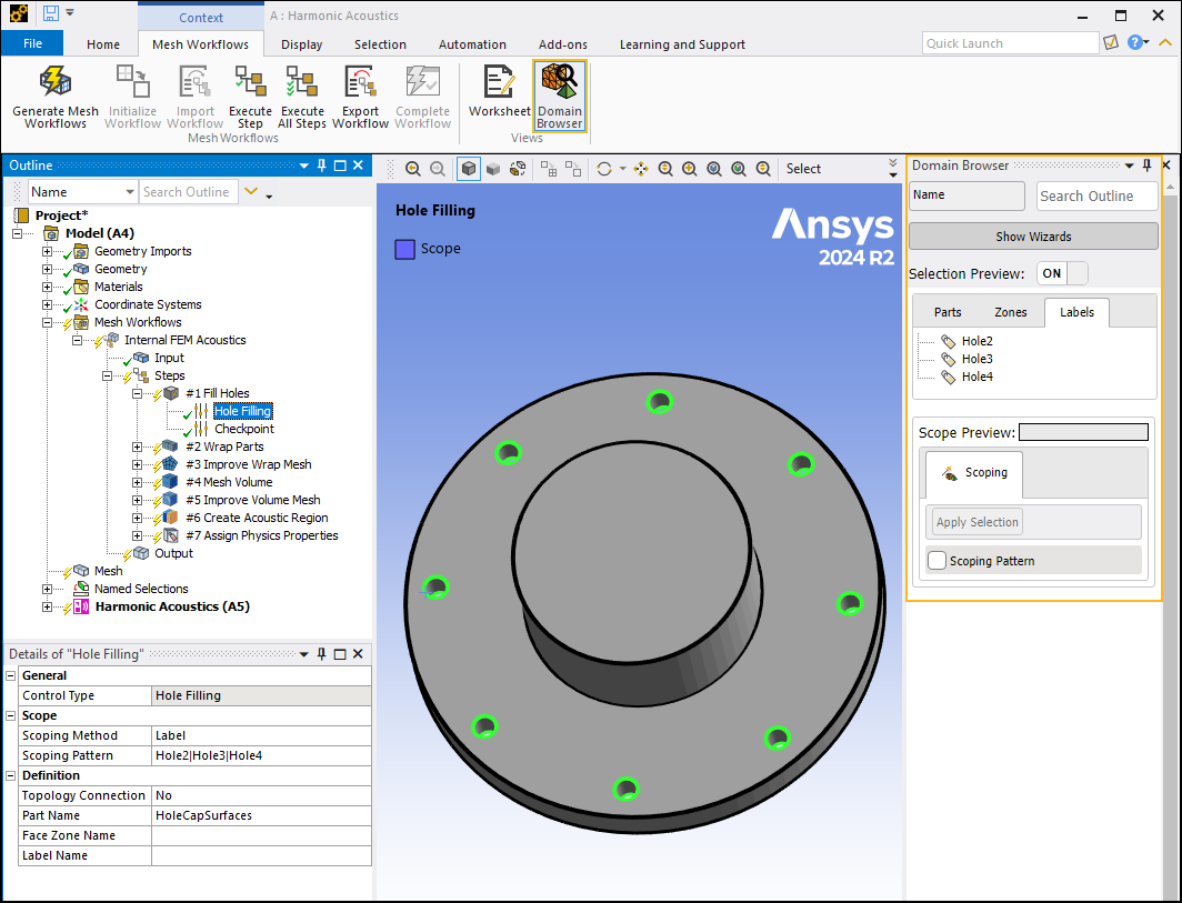
Mesh Workflows
Mesh Workflows has been enhanced to:
Provide Mesh Settings options to create the mesh based on acoustic settings.
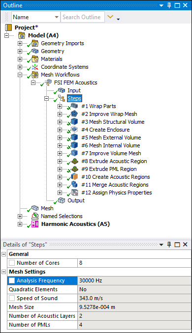
View model parts, zones, and labels involved in the mesh workflows using the Domain Browser that is available from the Mesh Workflows context tab. This feature also enables you to edit individual controls in mesh workflows.
Provide Quad Based Remeshing in the BEM Acoustics mesh workflow.
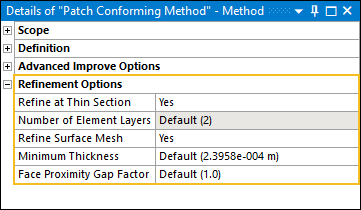
Tetrahedrons Mesh Method - Patch Conforming Algorithm
Now, when you specify a mesh Method as Tetrahedrons, and set the Algorithm property to Patch Conforming, a new Details pane category is available: Refinement Options. This category includes the property Refine at Thin Section. This property enables you to automatically refine the mesh in order to achieve two element layers in thin sections of the geometry. When active, this feature also provides an additional property, Refine Surface Mesh, that provides options to further refine the surface mesh in the vicinity of thin section to avoid very high aspect ratio elements.
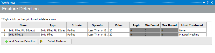
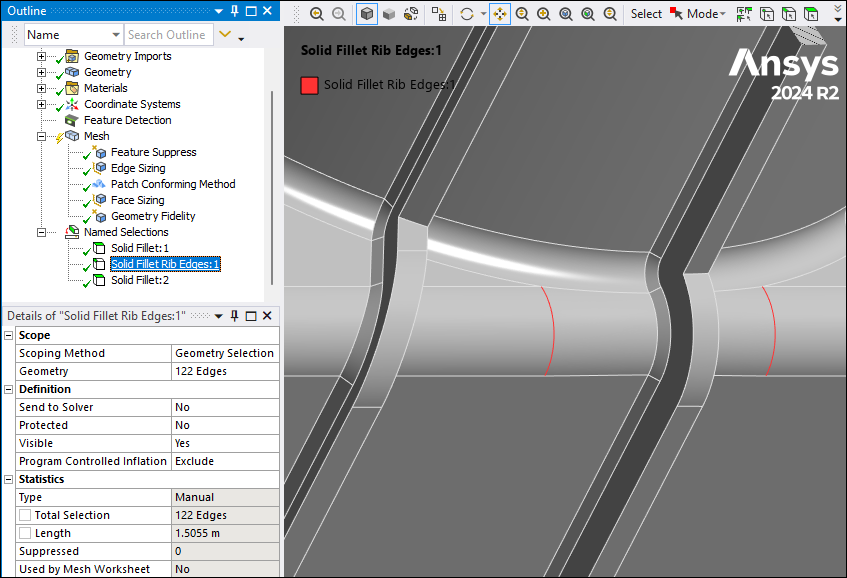
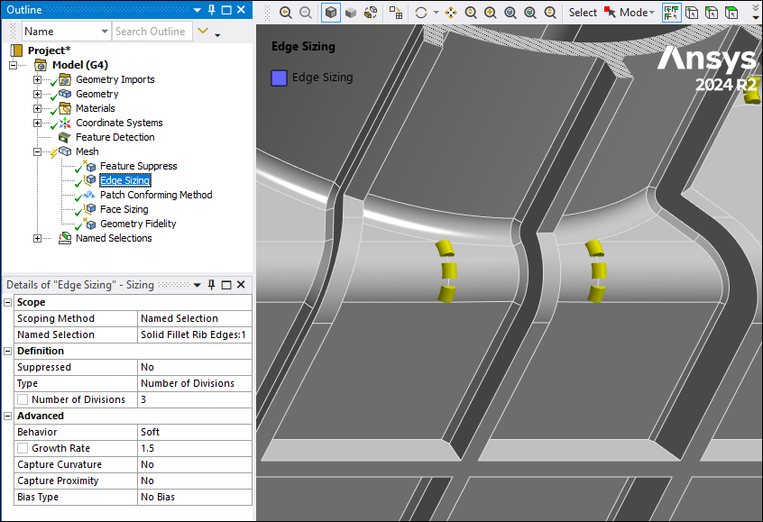
Feature Detection
The Mesh Quality Worksheet has been enhanced to provide mesh treatment for
Solid Fillet Rib Edges and Shell Fillet Rib Edges. These side edges
of fillets can then be added to Size Controls to request a specified number of elements
for mapped mesh faces.
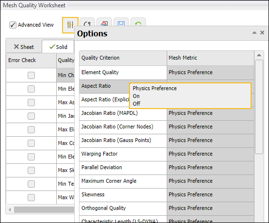
Mesh Quality Worksheet
Mesh Quality Worksheet has been enhanced to provide:
The ability to be used as a pure post-processing/visualization tool for mesh quality for all settings of Check Mesh Quality.
A right-click option to open the troubleshooting documentation to offer guidelines on how to fix poor quality elements in the mesh.
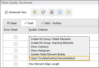
Options to increase or decrease the number of element layers displayed around warning/failed elements for the Quality Criterion contours.
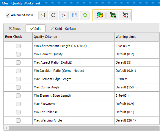
A new option to open a dialog box that enables you to customize the visible quality criteria.
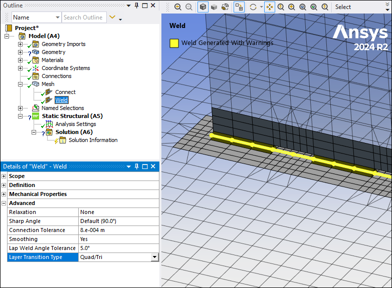
Weld
The Weld control has been enhanced to provide:
Solid-Solid weld connection for Mesh Independent weld.
Export > Weld Definition Files option from Weld object in the Outline.
Layer Transition Type to specify the mesh element type created during layer transition.


MultiZone Method
The MultiZone Method has been enhanced to provide a Program Controlled option under the Decomposition Type property to automatically determine decomposition type for each body and meshes them accordingly. For example, if bodies are detected as being thin, the Thin Sweep decomposition type will automatically be chosen.
Quad Layer
Quad Layer has been enhanced to:
Provide Auto-Defeature option to partially suppress edges close to holes, such as defeaturing that allows more quad layers to be created
Provide Preview option Quad Layer to preview the quad layers before mesh generation.
Layer Transition Type (see above) to specify the mesh element type created where quad layers terminate and connect to general quad dominant mesh. Three different pattern types are now available as seen in Weld section.
LS-DYNA System
Multi-Load Step Acoustic Simulation
You can use the BEM technology in the LS-DYNA Acoustics system coupled with a Harmonic Response analysis to create a Multi Load Steps Acoustic simulation. The following example illustrates the noise created by an e-motor for a BEM acoustics analysis.
Coupled Structural Thermal Electromagnetic Analysis
Using current or voltage loads, you can now simulate a Coupled Structural Thermal Electromagnetic analysis in the LS-DYNA system. In the following example of a fuse, currents are higher at the center where the cross section is smaller. The solver uses thermal expansion and erosion at high temperature to simulate a break of the fuse and as a result, an open circuit.
Analysis
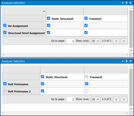
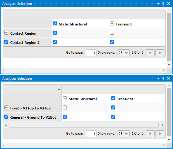
Analysis Selection for Model-Level Objects
For environments that use the Mechanical APDL solver and that are independent (no initial conditions) from other environments, the Analyses Selection worksheet now supports Material Assignment, Contact, and Joint objects in addition to Bolt Pretension load objects. For all of these object types, you can specify whether to include or exclude the corresponding data for a simulation using the Analyses Selection worksheet.
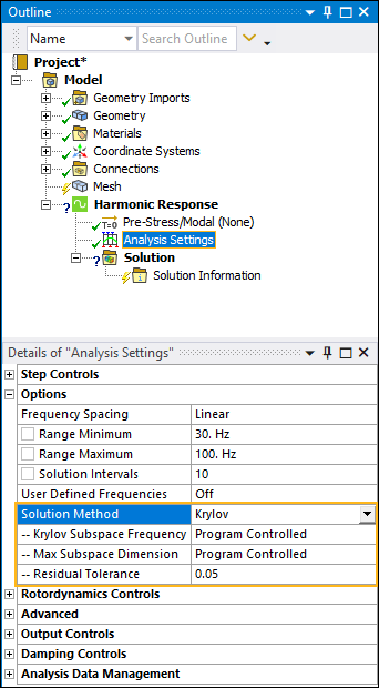
Krylov Solution Method
For pure acoustic Coupled Field Harmonic, pure acoustic Harmonic Acoustics, and Harmonic Response analyses, there is a new option for the Solution Method property: Krylov. The frequency-sweep harmonic analysis based on the Krylov method provides a high-performance solution for forced-frequency simulations in acoustic analyses. It can provide quick, estimated results compared to the Full method.
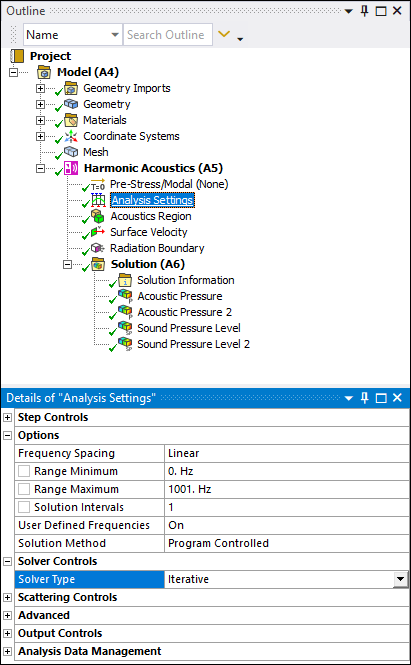
Iterative Solver Type Support for Harmonic Analyses
Now, you can use the Iterative solver (Analysis Settings > Solver Controls > Solver Type) for Coupled Field Harmonic (pure acoustics), Harmonic Acoustics (pure acoustics), and Harmonic Response analyses when the Solution Method property (Analysis Settings > Options) is set to Program Controlled or Full.
Acoustics Analyses
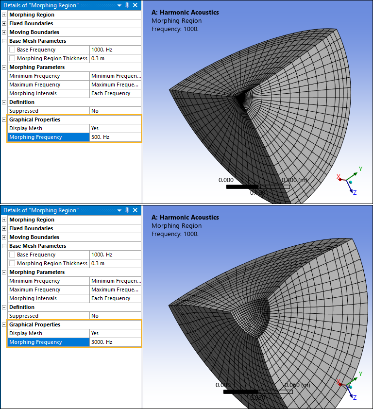
Harmonic Acoustics Adaptive Mesh Display
The Morphing Region object, available for Harmonic Acoustics analyses, now provides a new graphical display property: Display Mesh. You use this new option to display the adapted or "morphed" mesh of the Morphing Region, for a specified frequency value. You can change frequency values to review how the mesh adapts.
Coupled Field Analyses
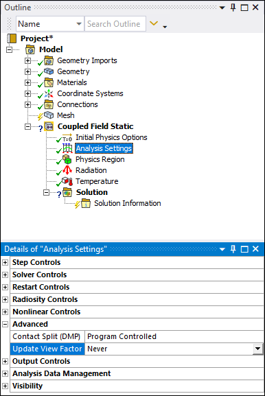
Update View Factor
Now, when you are performing a Coupled Field Static or a Coupled Field Transient analysis that specifies structural and thermal physics, the Advanced category of the Analysis Settings object includes a new property: Update View Factor. For each Radiation loading condition included in the analysis that has the Correlation property set to Surface to Surface, the application updates the view factors at the specified intervals. The use of this property requires that you specify large deflection and at least one Radiation load.
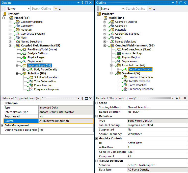
Importing Loads from Maxwell
You can now import Surface Force Density and Body Force Density loading conditions from the Maxwell application to downstream Coupled Field analyses.
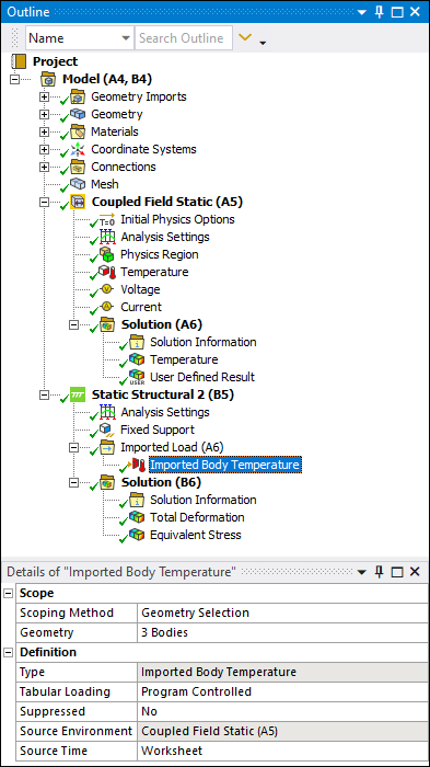
Imported Body Temperatures
You can now import temperatures from upstream Coupled Field Static or Coupled Field Transient analyses into downstream Static Structural or Transient Structural analyses.
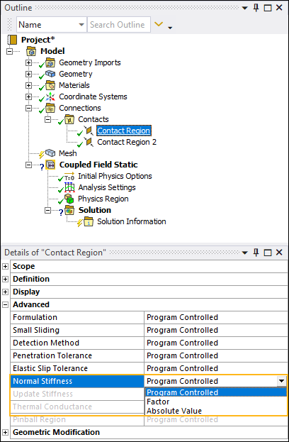
Normal Stiffness in Coupled Field Analyses
For electrostatic-structural Coupled Field Static and Coupled Field Transient analyses that include contact, you can now specify the Program Controlled setting for the Normal Stiffness property.
Structural Optimization
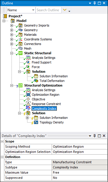
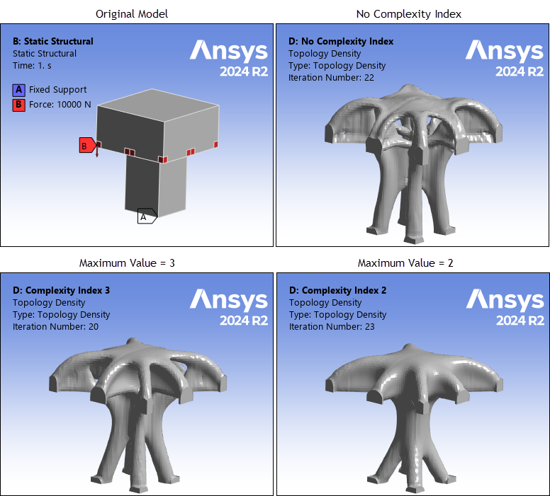
Level-Set Method Enhancement
A new Manufacturing Constraint is available: Complexity Index. This manufacturing constraint enables you to control the complexity of optimized designs and minimize the creation of overly complex structures.
For the following example, the design gets simpler (less perforations) as the complexity index is decreased.
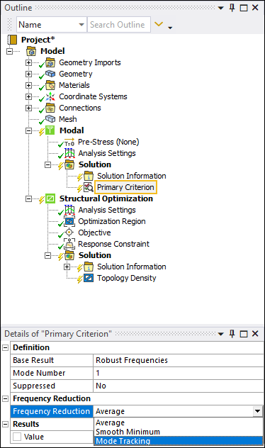
Primary Criterion for Modal Analyses
Now, when you specify a Primary Criterion object under the Solution object of a Modal analysis and set the Base Result property to Robust Frequencies, the Frequency Reduction property includes a new option: Mode Tracking. This option enables you to track an eigenmode of interest.
Mixable Density Optimization Method Enhancements
Upstream Harmonic Response analyses.
User Defined Criteria in upstream Harmonic Response analyses that you can use as a Response Constraint and Objective.
Stress criterion that you can use as a Response Constraint or Objective.
Shape Optimization Method Enhancements
Extrusions
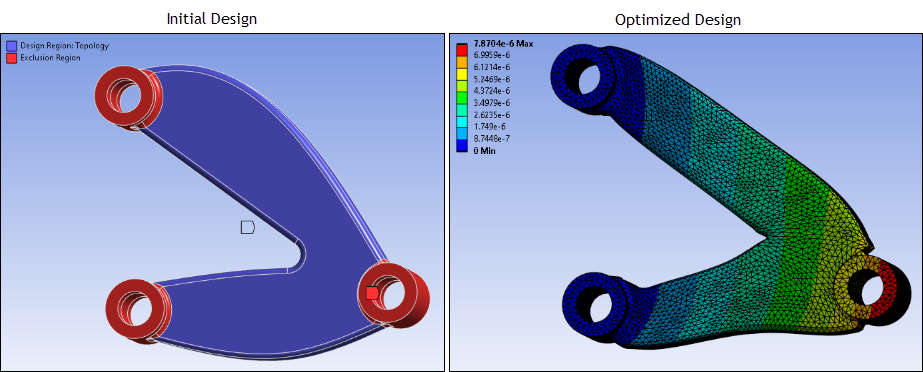
The Shape Optimization method now supports the use of the Extrusion Manufacturing Constraint.
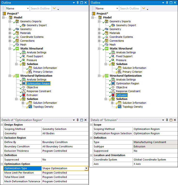
For example, using the extrusion constraint on the following model, you can reshape the body while forcing only in-plane deformation.
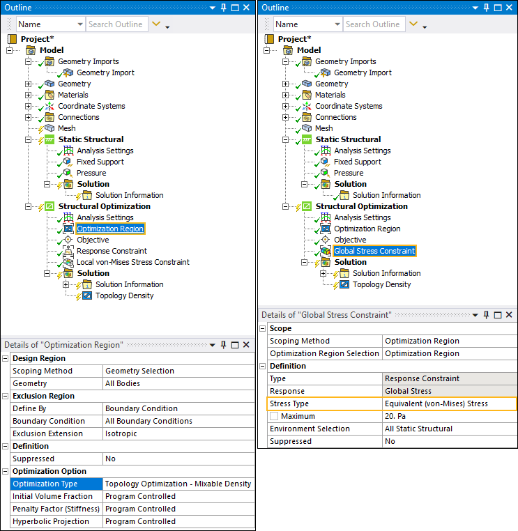
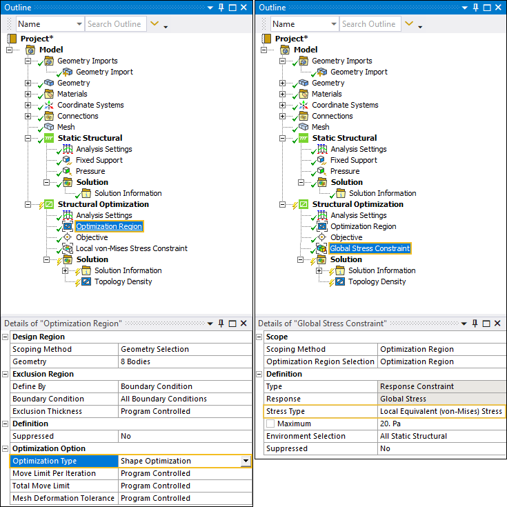
Local Equivalent von-Mises Stress Response Constraint
The Shape Optimization method now supports the Local Equivalent von-Mises Stress Response Constraint.
Fracture
Crack Initiation and Propagation using SMART Crack Growth
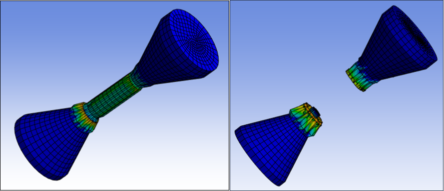
During a 3D Static Structural analysis, the Fracture analysis now provides a new object: Crack Initiation. You use this new object to specify a criterion for determining when the application initiates a crack in a specific region (or zone) of the geometry. You can also specify the location, orientation, and the size of the crack to be initiated. You apply this object and its definitions to a SMART Crack Growth object using the Initial Crack property, to study the crack propagation.
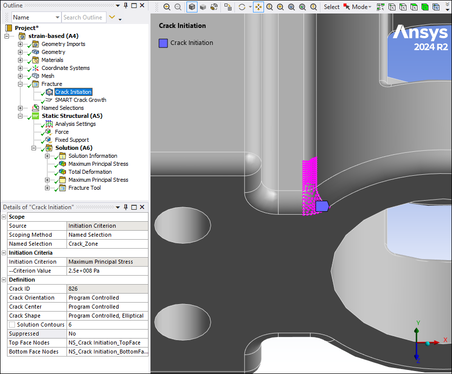
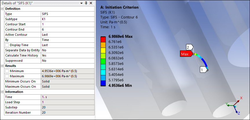
Here, a SIFS result shows the crack front contour created for the specified crack initiation criterion.
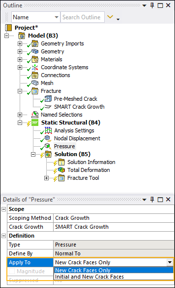
Applying Pressure on New Crack Faces (SMART Crack Growth)
For 3D Static Structural analyses, you can now scope a Pressure load to a SMART Crack Growth object.
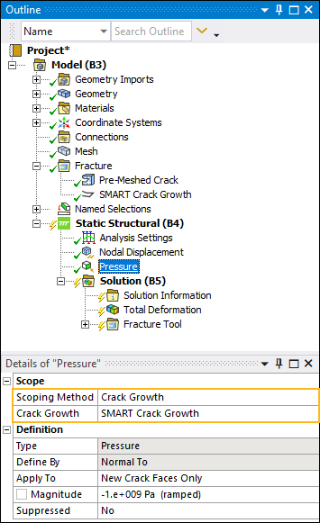
This enables you to apply the pressure to only the new crack faces the application generates during the smart crack growth process or to both the new and the initial crack faces of the crack associated with the SMART Crack Growth object.
Loads/Supports/Conditions
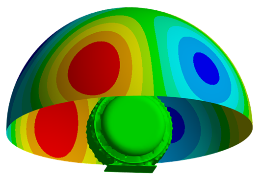
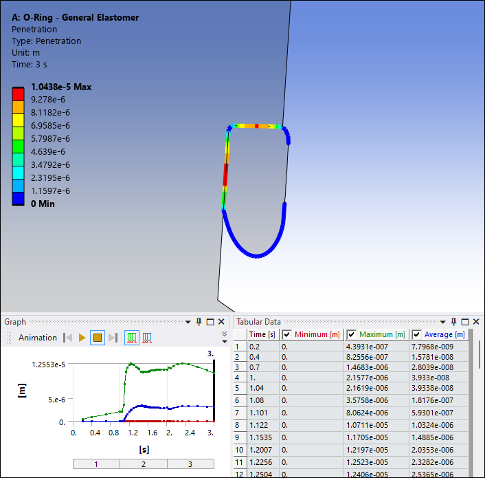
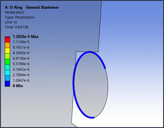
Fluid Penetration Pressure
For Static Structural analyses, there is a new loading condition available: Fluid Penetration Pressure. This loading condition enables you to simulate surrounding fluid or air penetrating into a contact interface.
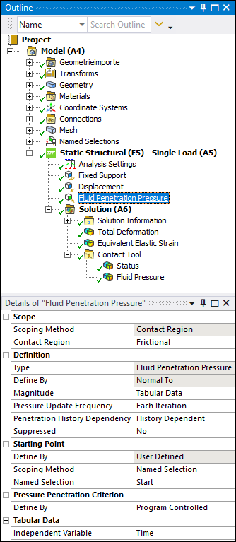
For example, here is a model of a sealing system, consisting of an elastomer O-ring, steel piston, and steel cylinder. The fluid penetration pressure is applied on the contact interface between the O-ring and piston.
Importing Load Data from External Data
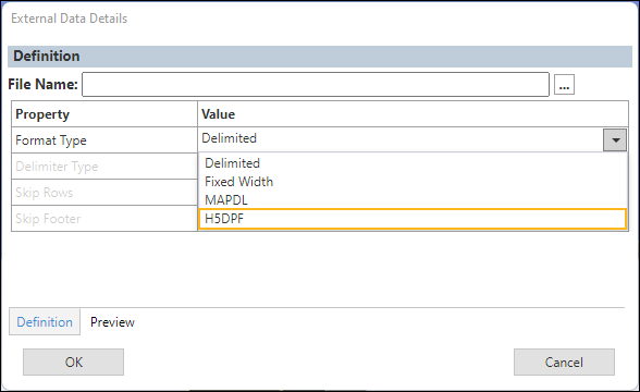
You can now use the External Data feature to import velocities from Hierarchical Data Format (HDF) Version 5 (.hdf5/.h5) files that contain the results and meshed regions from external solvers, such as MASTA, NATRAN, etc., using Imported Velocity. This feature is supported for Coupled Field Harmonic and Harmonic Acoustics analyses only.
The application generates this imported loading condition using the data processing framework (DPF) to generate a binary file from which the application maps the loading data.
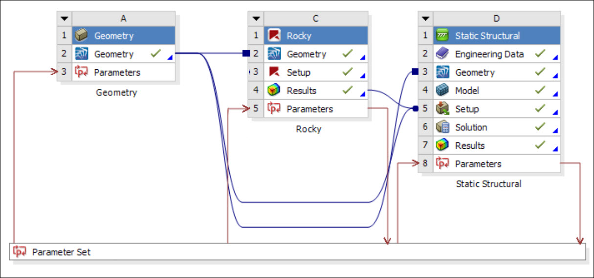
Importing Loads from Ansys Rocky
Now, when you import data from Ansys Rocky into Mechanical, the data for Imported Convection and Imported Force loads automatically populates the Data View worksheet for the given load object.
Imported Remote Loads
For a Maxwell analysis that includes a parametric sweep over RPMs, the Imported Remote Loads object/feature includes new properties:
Interpolate RPM. This property enables you to linearly interpolate the harmonic force and moment loads between two known RPM values with equal spacing. You can also specify custom spacing using a manually defined comma-separated values (.csv) file.
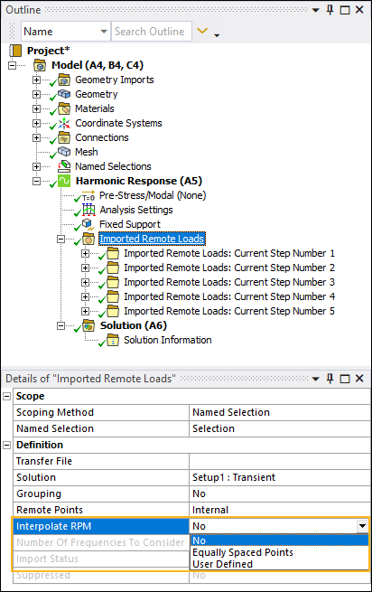
Filter by Order: This property enables you to import only required orders at every RPM.
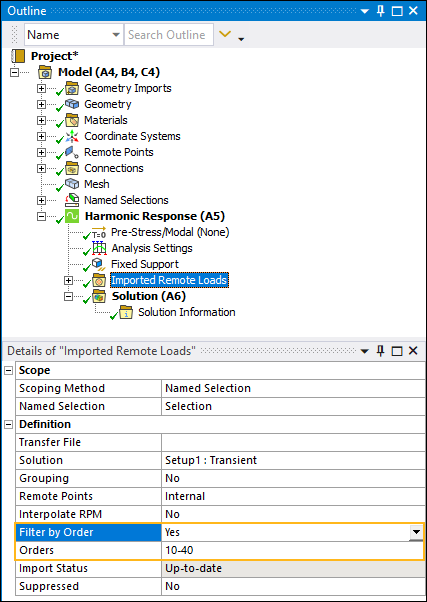
Data View Worksheet Additions for Submodeling and Results File Import
The Data View worksheet for Imported Temperatures and Imported Body Temperatures now supports the data properties Scale and Offset when importing boundary condition loads through the Submodeling and Results File Import features. These options enable you to modify imported temperature data by either multiplying the scale and/or adding an offset to the temperature values.
Solution
Resource Prediction
The Resource Prediction feature is now only supported with the Structures AI+ license. Additionally, the feature now:
Is supported for Full Harmonic Response analyses when the Solution Method property is set to either Full or Program Controlled.
Supports predictions for Static Structural analyses that include nonlinear conditions such as large strain or deformation, nonlinear material property definitions, as well as nonlinearities associated with contact conditions.
Performs predictions using the number of cores specified in the Solve Process Settings dialog. Previously, the application performed prediction and displayed table data based on a default core count of 4 cores.
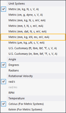
New Unit System
A new unit system is now available: Metric (mm, kg, kN, ms, mV, mA). All analyses that use this unit system and that have the Solver Target property set to Mechanical APDL, the application sets nmm for the Solver Unit System property (Analysis Settings > Analysis Data Management).
Results and Post Processing
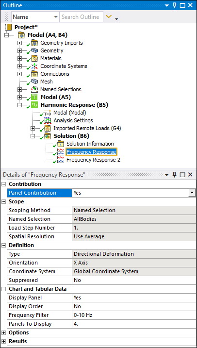
Panel Contribution
The Panel Contribution option now supports most Frequency Response results for Harmonic Response analyses.
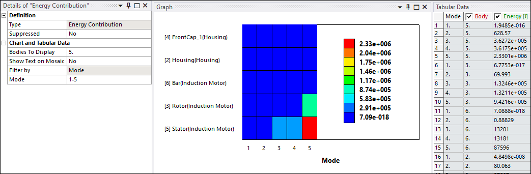
Energy Contribution
For Modal analyses only, you can now specify an Energy Contribution result for potential energies. This result produces a mosaic chart highlighting the potential energy for each body and every mode shape.
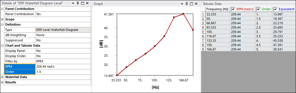
Waterfall Diagram Results
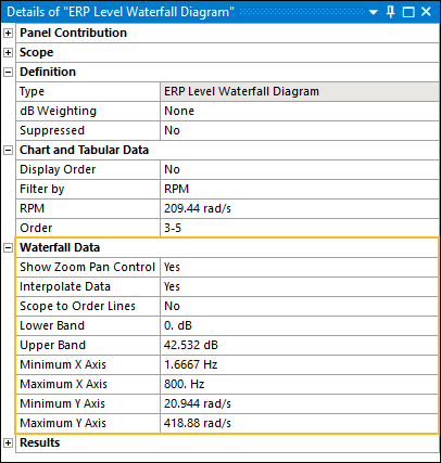
Several changes have taken place for waterfall diagram results:
Now, using the options of the Chart and Tabular Data category of the Details pane, you can simultaneously filter waterfall diagram results by RPM and Order so you can further refine the result data presented in the Graph and Tabular Data windows. In the previous release, you could only filter these results by RPM or Order.
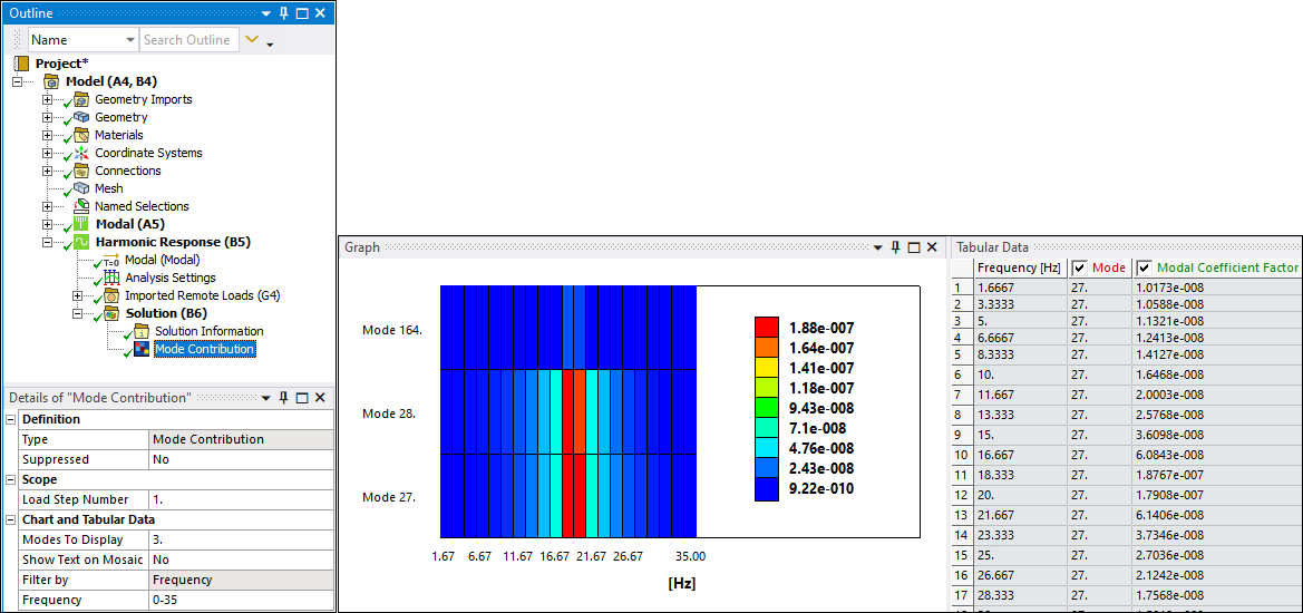
The Modal Coefficient Factors (MCF) Waterfall Diagram result has been renamed to Mode Contribution. You access this new result type from the new Contribution menu on the Solution tab for the supported analysis types.
The Details pane properties for waterfall diagram results are now available under a new category: Waterfall Data. Previously, these properties were included in the Chart and Tabular Data category. The behavior of the properties remains the same.
The Chart and Tabular Data category includes new filter properties (Display Panel/Display Order/Display Mode) based on analysis and result types. You can now display a mosaic chart for different contribution types. This enables you to perform targeted post processing by filtering complex response data to determine which bodies have the highest response at specific mode shapes and frequencies.
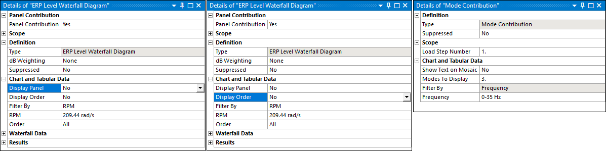
The Selection Mode property of the Chart and Tabular Data category has been renamed to Filter By. The options remain the same and include RPM and Order.
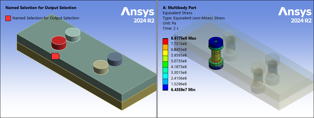
Write Results for Specific Named Selections Only
The Output Controls category of the Analysis Settings object includes a new property: Output Selection. This property enables you to store results only on specific geometry- or meshed-based Named Selections in order to reduce the size of your result file. You set this property to By Named Selection and specify your desired named selection(s).
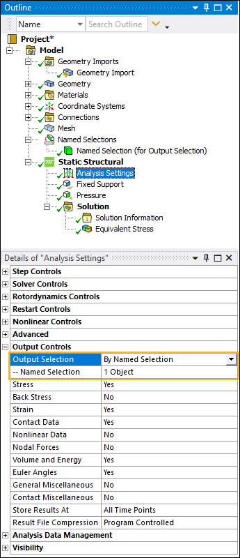
Once you solve the analysis, results are only stored for the geometry or mesh entities of the Named Selection.
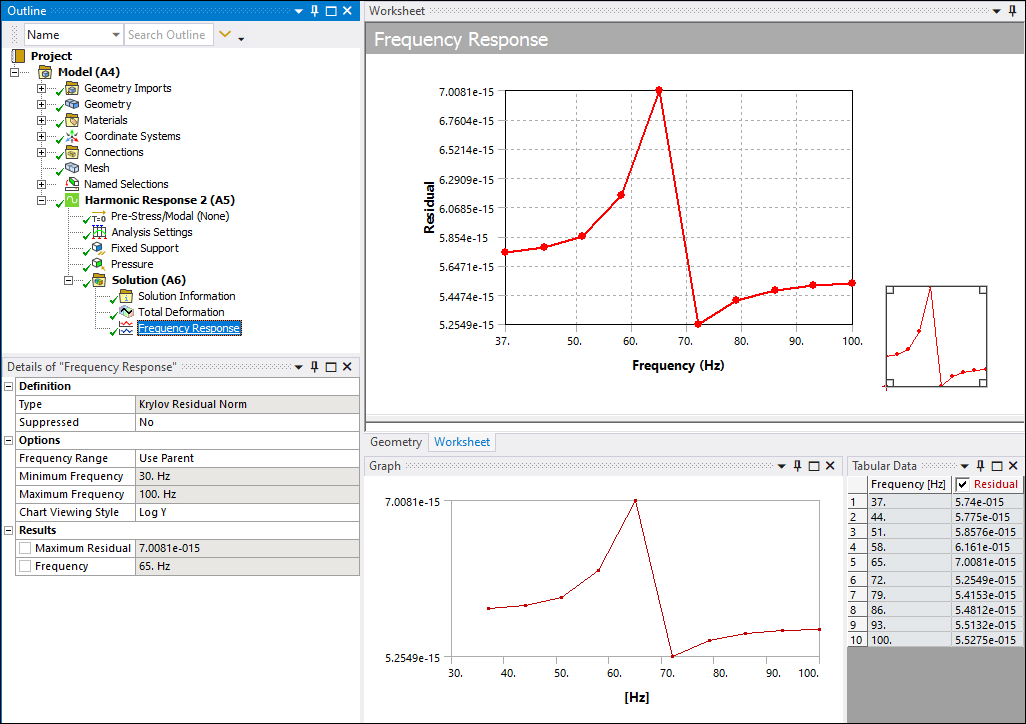
Krylov Residual Norm
Now, when you solve a pure acoustic Coupled Field Harmonic, pure acoustic Harmonic Acoustics, or Harmonic Response analysis using the Krylov option of the Solution Method property, a new Frequency Response result is available: Krylov Residual Norm. This result plots error estimations (residuals) across a frequency range for the harmonic distribution. The plot can provide information about how to best split the whole frequency range into multiple ranges.
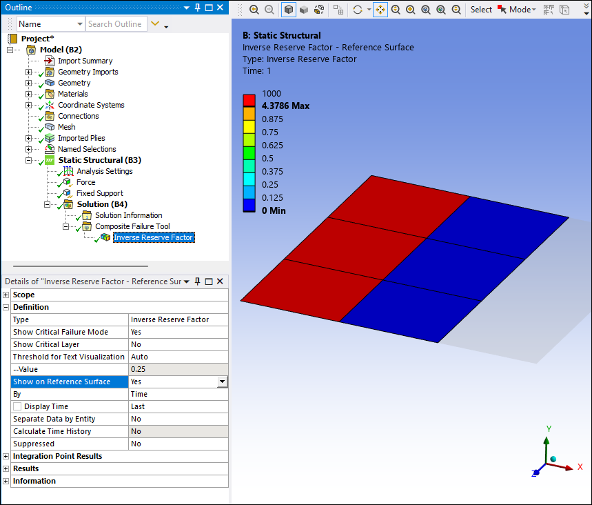
Composite Failure Tool
The Composite Failure Tool includes a new property: Show On Reference Surface. This property enables you to display the worst failure, per solid stack, on the shell mesh of the specified Reference Surface only.
Python Result
When you insert a Python Result, the worksheet automatically includes default script content. In previous releases, this script content was based on the Total Deformation result. Now, the content depends on the type of analysis to which you have added the result.
Add-ons
DesignLife
DesignLife now offers a Frequency Selection Method for frequency-domain loading events and the selection of existing Harmonic and Modal systems for Environment definition. Temperature is available for stress and strain analyses and Shell Layer, Seam Weld Location and Seam Weld Type results can be displayed for Shell Seam Weld analysis.
NVH Toolkit
Transfer Path Analysis (TPA) functionality has been added to the FRF Calculator. The MAC Calculator now supports cyclic symmetry and coordinate transformation for RST to RST comparison.
Restart Analysis
Restart Analysis is a new addition to the Add-ons Ribbon. This add-on makes Static-Static or Transient-Transient structural restart capabilities available within the Mechanical environment.

Additional Localization Support
Additional localization support is available for the Restart Analysis and Forced Response add-ons. These add-ons now support Chinese, Japanese, German, and French languages as well as varied decimal separators.
Motion
Condensed Part and Imported Condensed Part
Motion now allows the use of Condensed Part and Imported Condensed Part objects, including support for contact with a Condensed Part.
Velocity and Acceleration Waterfall Diagrams
Velocity and Acceleration Waterfall Diagrams are now available for Motion analyses, using a Short Time Fourier Transform (STFT) algorithm.
Spline Data View
Data View is now available for Spline objects, allowing rapid entry of large amounts of data via copy and paste.