


For a general discussion of acoustics analyses in Mechanical, see Acoustics Analysis Overview.
Introduction
Like the Harmonic Acoustics analysis, the LS-DYNA BEM (Boundary Element Method) Acoustics analysis is used to determine the frequency response of a structure and the surrounding fluid medium to loads and excitations that vary sinusoidally (harmonically) with time. However, the fluid region in the BEM method is not meshed. The BEM is a numerical computational method of solving linear partial differential equations which have been formulated as integral equations (in boundary integral form).
The integral equation may be regarded as an exact solution of the governing partial differential equation. The boundary element method attempts to use the given boundary conditions to fit boundary values into the integral equation, rather than values throughout the space defined by a partial differential equation. Once this is done, in the post-processing stage, the integral equation can then be used again to calculate numerically the solution directly at any desired point in the interior of the solution domain.
Points to Remember
Note that:
This analysis type supports 3D geometries only.
Only shell bodies can be used. Material and thickness of shell bodies have no influence on the result. The fluid domain is not represented.
The results supported for this type are Contour, (Pressure, Total Velocity, Sound Pressure Level) and Frequency (Pressure, Sound Pressure Level, Directional Velocity).
Check Acoustic Mesh Size
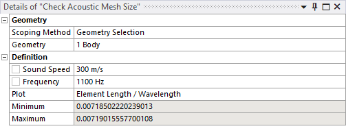
The Check Acoustic Mesh Size object enables you to evaluate the ratio of the element length to acoustic wavelength. The element length is a property of each element of the mesh. The acoustic wavelength is defined as Sound speed/frequency. It is recommended that you use a ratio of less than 1/8.
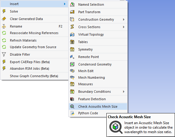
To insert a Check Acoustic Mesh Size object, right click the Model object and select . Alternatively, you can click the Check Acoustic Mesh Size icon found in the Acoustics section of the Environment tab of the ribbon.
Once you have inserted the object, scope it to the body of interest and enter the Sound Speed and Frequency values. The Minimum and Maximum fields show the minimum and maximum ratios of the Element lengths to the Wavelength.
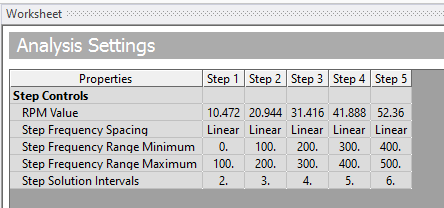
Establish Analysis Settings
The Analysis Settings object contains several fields that are specific to performing and acoustics analysis using LS-DYNA.
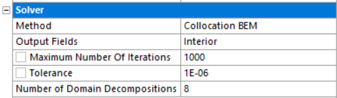
- Method
The options available for this property are:
Program Controlled
Program controlled sets the Method based on the Output Fields value:
for an Exterior output field, the solver uses the Variational Indirect BEM method.
for an Interior output field, the solver uses the Collocation BEM method.
Variational Indirect BEM
An indirect BEM implemented by variational formulation for solving the Helmholtz integral equation. In this method, the primary variables are discontinuity of acoustic pressure and the normal gradient of the pressure across the boundary elements. This method is flexible and can work with acoustic problems with closed boundary and those with openings and appendices.
Collocation BEM
A direct BEM implemented by collocation formulation for solving the Helmholtz integral equation. In this method, the primary variables are the acoustic pressure and acoustic velocity. It works for closed boundary acoustic problems. The acoustic results (acoustic pressure, normal velocity, and acoustic intensity) can be obtained on the boundary elements directly.
Collocation BEM with Burton-Miller formulation
A dual collocation BEM based on a linear combination of the Helmholtz integral equation and the normal derivative of the Helmholtz integral equation (Burton-Miller formulation). This method can be used to eliminate the fictitious resonance (or non-uniqueness) for exterior acoustic problems.
- Output Fields
The space in which the output is calculated. Specify Interior if you have an enclosed domain or Exterior if you have an infinite domain.
- Maximum Number of Iterations
Specify the maximum number of iterations to reach convergence. The default value is 1000.
- Tolerance
Specify the convergence tolerance. The default value is 0.000001.
- Number of Domain Decompositions
Specify the number of domains that you want to divide the geometry into during the solution. Domain decompositions is used to save memory. For large problems, the boundary mesh is decomposed into the number of domains specified for reduced memory allocation. The default value is 8.
Note: If the Multiple Steps property is enabled under Step Controls, the Worksheet will be read only. The values are populated from the Imported Velocity object in the Outline. Only one active object is allowed and will populate the worksheet.
When you modify RPM properties in the upstream system (Harmonic Response), you must perform these 2 steps in order to update the RPM properties in the LS-DYNA Acoustics system:
Update the Setup cell of LS-DYNA Acoustics system in the project Schematic.
Right-click the Imported Load Group in the LS-DYNA Acoustics System and select Create velocities and Sync Analysis Settings.
.