This section covers special workflows and solution methods information. Some of the topics here include:
Descriptions of how the LS-DYNA system can interact with other Workbench systems.
SPH and Incompressible SPH Workflows
A Steady-State or Transient Thermal analysis system can be directly linked to an LS-DYNA system to import the calculated temperatures and provide thermal stress. For information on setting up this transfer, follow the description of how it is done for a structural system in Thermal-Stress Analysis in the Mechanical User's Guide
Note:
Imported temperatures cannot be scoped to beams.
LS-DYNA requires the definition of the Instantaneous Thermal Expansion Coefficient on materials to calculate thermal deformations.
A CFD analysis system can be directly linked to an LS-DYNA system to import the Temperature results from a heat transfer CFD analysis as body temperature loads. For information on setting up this transfer, follow the description of how it is done for a structural system in Using Imported Loads for One-Way FSI in the Mechanical User's Guide.
A CFD analysis system can be directly linked to an LS-DYNA system to import the Pressure results from a CFD analysis as imported pressures loads. For information on setting up this transfer, follow the description of how it is done for a structural system in Using Imported Loads for One-Way FSI in the Mechanical User's Guide.
When the Solver Type analysis setting is set to Coupled Structural Thermal Analysis, the LS-DYNA system in Mechanical supports thermal boundary conditions and results. The addition of these boundary conditions enables strongly coupled structural-thermal calculations, in support of simulations like frictional heating, battery abuse, or other analyses where mechanical and thermal solutions affect each other strongly.
The LS-DYNA system provides support for the following thermal loads in Mechanical: Temperature, Convection, and Heat Flux. These loads are implemented, respectively, with the keywords *BOUNDARY_ TEMPERATURE, *BOUNDARY_CONVECTION, and *BOUNDARY_FLUX. The system also supports Temperature and Heat Flux results, and the Temperature Tracker. Refer to the object descriptions for usage notes for LS-DYNA systems.
LS-DYNA provides two types of ALE solvers:
The unstructured ALE solver, which can be defined within Mechanical by assigning an ALE Method type. The unstructured mesh is created within Mechanical and is passed directly to the solver.
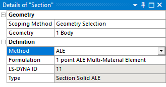
The structured ALE (S-ALE) solver can be invoked by creating a body with rectilinear box geometry and a Reference Frame set to S-ALE Domain. The default material for the domain is associated directly with the body. Additional bodies with Reference Frame set to S-ALE Fill, are filled into the S-ALE Domain. This is achieved by first meshing the S-ALE Fill bodies using the standard Mechanical meshing process. The surface meshes of these bodies are passed to the solver as dummy rigid shell bodies and are used to define the material with the S-ALE Domain. Once the filling is complete, the dummy rigid shell bodies have no further effect on the simulation. For more information, see the Initial Volume Fraction Geometry keyword.
The S-ALE Mesh Object is used to define mesh parameters and view the surface mesh for the S-ALE mesh that will be created within the solver.
Several objects are available for use in the ALE workflow:
The Coupling object which is added under connections, enables the setup of ALE-Lagrange interactions.
The ALE Boundary Object allows you to define stick and slip boundary conditions on the external faces of the ALE domain.
Note:
The mesh created within Mechanical is not directly used for the S-ALE domain. By default, the bounding box of the geometry and the number of elements generated by the Mechanical meshing process are used as parameters to define the size and density of a uniform rectilinear mesh that will be created by the solver. Further details are given in S-ALE Mesh.
Results for S-ALE bodies are not displayed on the original mesh. Instead, a mesh is reconstructed for each material associated with the original body to which the result object is scoped.
The reconstruction of the mesh is approximate and includes:
Finding the exterior surface of each material in its current location in the S-ALE domain. This is achieved by forming an isosurface on the volume fraction of each material in a cell (at 50%).
Filling the interior of the material with cells from the S-ALE domain that are completely inside the material.
Reconstructing an unstructured mesh for any gaps between the exterior surface and interior cells.
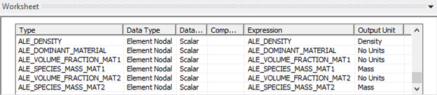
When ALE bodies are included in the model, several ALE-specific result variables are available as user defined variables: Density, Volume Fraction, Dominant Material, and Species Mass.
LS-DYNA provides a Smooth Particle Hydrodynamic (SPH) solver. The state of the system is represented by a set of particles which possesses material property and interact with each other within the range controlled by a weight function. Particle approximation is a truly mesh-free explicit Lagrangian method.
The SPH solver is a good choice in the following types of analyses:
Large material distortion—for example, crashworthiness, hyper-velocity impact
Moving boundaries, free surface—for example, fluid and structure interaction
Adaptive procedure—for example, forging and extrusion
To use this solver, your project must use a Reference Frame of type Particle and include a Particle Method mesh object.
For additional information about setting up an SPH analysis, see the following topics:
Note:
The default contact thickness between SPH parts and Lagrangian parts is zero. In some situations, it's recommended that you define a contact thickness in order to detect and avoid penetration between an SPH part and a Lagrangian part. If you set Contact Thickness to Yes in the SPH Controls section of the Analysis Settings, the solver will automatically define a contact thickness.
The SPH part viscosity can be set by scoping the SPH part to an Hourglass Control object and entering the Quadratic and Linear Viscosity. See *Hourglass for more information.
The Incompressible SPH (ISPH) solver allows you to solve FSI problems that involve structural and fluid bodies. Here is some general guidance for setting up an ISPH analysis using a Mechanical LS-DYNA system.
The fluid part must be a solid body with a Reference Frame of type Particle and you must mesh it with the Particle Method mesh method. To set the material of the fluid part you must scope an ISPH Region object to the body, set the Type to fluid, and enter the material properties of the fluid.
If a solid structural body is used in the model, you must extract its skin (using a modeling program like SpaceClaim) and define it as a new rigid shell body. The shell body should be meshed with triangles, then an ISPH Region should be scoped to the shell body. The interaction surface of the shell body is meshed with SPH particles using the ISPH Region. The ISPH Region will discretize the surface to SPH particles within the solver.
The interaction between the structure and the fluid is handled by the particle formulation of ISPH (particles can't overlap). No contact object is needed since the contact will be handled by the SPH particle formulation. The interaction occurs between the particle meshing on the surface of the structure (shell) body and the particles of the fluid region (solid body).
The Result worksheet shows results for SPH particles that are created inside the solver. See Post-processing for Solver-Created SPH Elements.
ISPH is suitable for slower fluid-flow simulations such as automotive water wading and gear box lubrication.
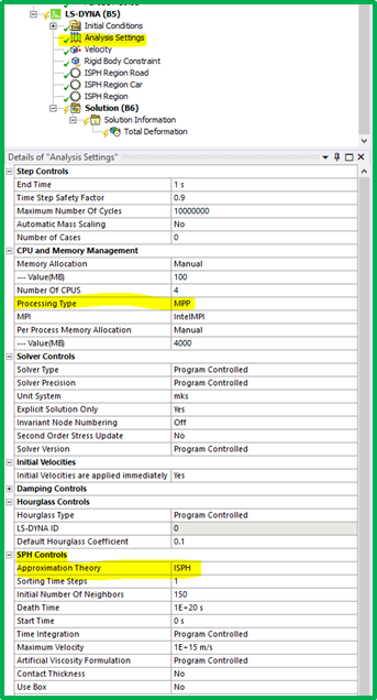
Note: ISPH is only available for an MPP simulation. You must set the processing type to MPP in the CPU and Memory Management section of the Analysis Settings Details panel in order to use it.
For additional information about setting up an SPH analysis, see the following topics:
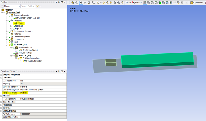
The following is an example of how to use the ISPH feature in the Workbench LS-DYNA system. The screen shots show an example of a car traveling through a puddle, but the steps describe the general procedure that you can use for any ISPH analysis.
Import an external CAD file containing the model into the LS-DYNA system.
Set the Reference Frame of the solid body that represents the SPH body to Particle.
Set the Stiffness Behavior of the ISPH surface bodies to rigid.

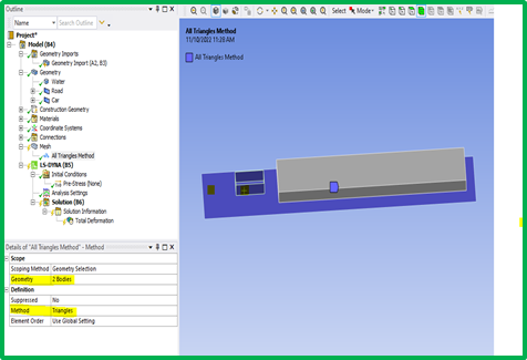
Insert a Mesh Method and scope it to the ISPH surface bodies. Set Method to Triangles so that you mesh the ISPH surfaces with triangles. Insert a Body Sizing object under Mesh and set a size for the triangle elements.
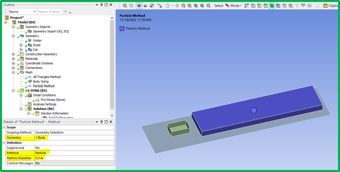
Add a Particle Mesh method and scope it to the SPH solid body. You can set the diameter of the particles.
Insert any necessary boundary conditions.
Insert an ISPH Region for each of the bodies in the analysis. Scope one region to each body. Set the Type (physics type) to Solid (for the shell bodies) or Fluid (for the solid SPH body) as appropriate and set the corresponding properties for each Region.

In the Analysis Settings properties, under CPU and Memory Management set the Processing Type to MPP, and under SPH Controls set the Approximation Theory to ISPH.
The setup of the ISPH analysis is complete. Add any additional objects that you need and you are ready to solve the model.
LS-DYNA provides two types of Smoothed Particle Galerkin (SPG) solvers:
The standard SPG solver used in the simulation of destructive manufacturing process such as riveting, screwing, drilling, and machining.
The Incompressible SPG (ISPG) Solver used for the simulation of incompressible free surface fluid flow such as the reflow process of solder joints in electronic equipment.
SPG and ISPG are mesh-free methods that use a finite element mesh, unlike SPH which requires the generation of a specific particle mesh. The SPG and ISPG bodies must be solid.
To apply SPG or ISPG methods on a part, scope the part in a section object with the method property set to SPG or ISPG. Additional information on SPG and ISPG are described in the following items:
To handle the interaction between a finite element part and an ISPG part, there is a new coupling object called ISPG to Surface Coupling. For additional information on this object, see:
To use the ISPG solver, the Solver Precision in the Analysis Settings must be Double and the mesh for the ISPG body must use tetrahedral elements. If these two conditions are not met, error messages that indicate the problem will be generated.
When you are using MPP for an SPG analysis, the card *CONTROL_MPP_DECOMPOSITION_PARTS_DISTRIBUTE is written to the input file. This card specifies the ID of a *SET_PART_LIST that includes all SPG part IDs. For further details, see *CONTROL_MPP_DECOMPOSITION_PARTS_DISTRIBUTE in the LS-DYNA Keyword and Theory Manuals.
When the Solver Type field in Solver Controls category of the Analysis Settings object is set to Coupled Structural Thermal Electromagnetic Analysis, the LS-DYNA system in Mechanical lets you perform an analysis using electromagnetic boundary conditions to evaluate the resistive heating effects in the model. When this solver type is selected, the Analysis Settings object provides EM Solver Controls and EM Step Controls categories with additional options.
Note:
The only EM solver type currently available is Resistive Heating.
The only unit system currently available for the EM workflow is MKS.
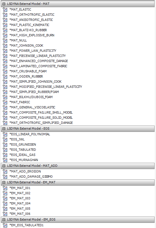
Electromagnetic material properties can be added to materials from Engineering Data in Workbench. The native electric properties supported are: Isotropic Resistivity, Orthotropic Resistivity, and Isotropic Relative Permeability. In Engineering Data, you can also select LS-DYNA cards to add electromagnetic properties to materials. The cards are EM_MAT_001, EM_MAT_002, EM_MAT_003, EM_MAT_004, EM_MAT_005, EM_MAT_006, and EM_EOS_TABULATED1.
The LS-DYNA system provides support for the following Mechanical electromagnetic loads: Voltage and Current. These loads are implemented with the keyword *EM_BOUNDARY_ PRESCRIBED.
The LS-DYNA BEM (Boundary Element Method) Acoustics analysis is used to determine the frequency response of a structure and the surrounding fluid medium to loads and excitations that vary sinusoidally (harmonically) with time. However, the fluid region in the BEM method is not meshed. The BEM is a numerical computational method of solving linear partial differential equations which have been formulated as integral equations (in boundary integral form).
Since the LS-DYNA Acoustics system shares much of its functionality with the Mechanical Harmonic Response system, the system is primarily documented in LS-DYNA Acoustics Analysis in the Mechanical Acoustic Analysis Guide. Included here is a discussion of how to import a velocity into an LS-DYNA Acoustics analysis because currently it cannot be done directly.
Velocity Import
To import velocities into an LS-DYNA Acoustics system you must use a Harmonic Response analysis as described here.
In the Workbench Project Schematic, link a Harmonic Response system to an LS-DYNA Acoustics system.
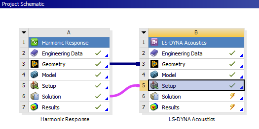
The application automatically inserts an Imported Velocity object into the downstream system.

See Applying Imported Boundary Conditions in the Mechanical User's Guide for more information. The Imported Velocity uses the new Load Mapping Workflow Specification. For more information regarding the properties of the Imported Velocity object, see Imported Load (Group) in the Mechanical Object Reference.
The Analysis Settings options such as RPM Value, Step Frequency Range Minimum, Step Frequency Range Maximum, and Step Solution Intervals are set based on the Specify RPM, RPM Selection, and Source Frequency values in the Imported Velocity object.
The LS-DYNA Workbench system uses default solver settings for some LS-DYNA Control Cards (keywords starting with *CONTROL) and for some settings affecting the results file content (keywords starting with *DATABASE).
These settings are not available in the user interface, nor are they written when the corresponding option is set to Program Controlled. If you wish to use different default settings, set the option Default Solver Control Cards located under Advanced in the Analysis Settings Details panel to Omit, which will omit these default solver cards. By default, the option is set to Keep.
*CONTROL_TERMINATION and *DATABASE_BINARY_D3PROP are the only cards written when Omit is selected. You can provide your preferred settings by using Keyword Snippets.
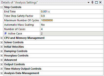
The *CASE command enables running multiple LS-DYNA analyses or cases sequentially by submitting a single input file. For further details, see *CASE in the LS-DYNA Keyword User's Manual. The LS-DYNA system includes several options to support the setup of a multiple case workflow.
The Number of Cases property is set under the Step Controls section of Analysis Settings. This property defines the number of cases. When greater than 0, the CASE input argument is passed to the solver to enable initialization of a multiple case solve. The default value is 0, which indicates that the *CASE command is not active.
The Active Case property is set under Step Controls section of Analysis Settings. This property defines the currently active case. The default value is 0, which indicates that all cases should be solved. If a case number between 1 and Number of Cases is specified, then only that case will be solved. In this scenario, the Case Number property set under the result objects becomes hidden and the result retrieved will be for the Active Case. The Active Case property is parameterizable. When set, each case is treated as a separate design point which, with the appropriate settings in Workbench, allows the cases to be solved simultaneously.
The Case Number can be set under the following objects:
Initial Conditions (Velocity, Angular Velocity, Drop Height)
Fixed Support
Displacement
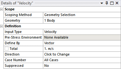
Velocity
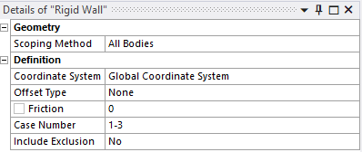
Rigid Wall
This property provides the option to select a case number between 1 and Number of Cases specified under Analysis Settings. The input string accepts a comma separated list of case numbers and/or ranges of case numbers. It should be of the form a, b-c, d, where a, b, c, d are integer case numbers, b-c represents the range of case numbers from b to c. For example:
Case Number = 1-3 (Load applies to case 1, 2 and 3)
Case Number = 1, 3 (Load applies to case 1 and 3)
Case Number = 1-2, 4-5 (Load applies to case 1, 2, 4, and 5)
This field indicates the case numbers for which the object is active. In the input file, the keyword corresponding to the object is wrapped in the *CASE_BEGIN_N and *CASE_END_N keywords to indicate to the solver that it must be applied to that specific case. The default value is All Cases, which means the keyword corresponding to the object will be applied in all cases.
Note: At least one object (for example, Velocity or Rigid Wall) must be defined for each case from number 1 to Number of Cases, otherwise the solver will report an error.
When running a multiple case solve, a separate set of result files is created for each case. The Case Number property is set under the result object. This property provides the option to select a case number between 1 and Number of Cases specified under Analysis Settings. The default value is 1, which indicates that the result shown is for the first case.
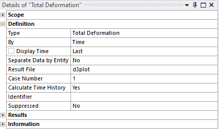
Note: The Worksheet data shown by selecting Solution Output under Solution Information is for the first case only.
A multi-system analysis is a set of linked LS-DYNA analyses. Each analysis runs the solver with a regular input file but with some additional initialization using data from an upstream (preceding) LS-DYNA analysis. The data available for initialization to a downstream LS-DYNA analysis includes the deformed geometry positions and stress state. The data used to initialize subsequent analyses is passed to the solver via the binary dynain.lsda file.
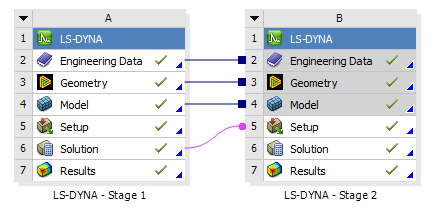
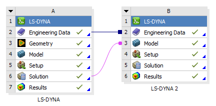
This process has similarities to the full restart described in section Restarting an LS-DYNA Analysis and also the sequential solution described in section Explicit-to-Implicit Sequential Solutions. There are two methods for connecting the sequential LS-DYNAj systems, one where the model is shared by both systems, and another where the solved model from the first system becomes the initial model for the second system.
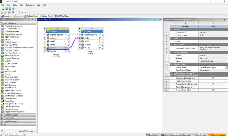
This section describes how to setup a two-system simulation using shared model data. In this case the Solution cell from the first system is linked to the Setup cell for the second system.
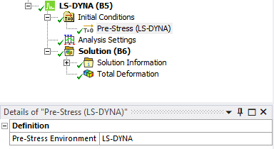
Linking two LS-DYNA systems in this way results in the automatic creation of a Pre-Stress initial condition in the Analysis for the second system. This indicates that data is to be transferred between the systems.
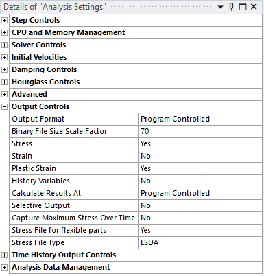
In order to enable the transfer of data a dynain.lsda file must be generated by the analysis of the first system. This is achieved by setting the property Stress File for flexible parts to Yes under the Output Controls section of Analysis Settings. By default, the dynain file is created in the LSDA format. There is an option to switch this to ASCII and Binary. However, the multi-system workflow does not currently support using either of those formats. The default settings are to transfer data for only flexible bodies. This behavior can be customized using the Dynain Output Controls object described below.
|
|
|
The dynain.lsda file is automatically copied from the system one analysis to the system two analysis and submitted to the solver via the *INCLUDE keyword in the system two input file.
This procedure can be extended to include additional systems as required.
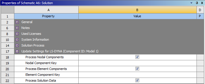
This section describes how to setup a two-system simulation using the results of the first solution to initialize the model of the second solution. In this case the Solution cell from the first system is linked to the Model cell for the second system.
In order to properly transfer the deformed geometry and stresses, you need to select the Process Solution Data check box in the Properties of the first LS-DYNA system. The data can only be transferred at the end of the solution, not at an earlier point in the solution.
Note: The unit systems used by the downstream systems must be the same as the unit system of the upstream system. If the unit systems are different an error is generated.
In order to enable the transfer of data a dynain.lsda file must be generated by the analysis of the first system. This is achieved by setting the property Stress File for flexible parts to Yes under the Output Controls section of Analysis Settings. By default, the dynain file is created in the LSDA format. There is an option to switch this to ASCII and Binary. However, the multi-system workflow does not currently support using either of those formats. The default settings are to transfer data for only flexible bodies. This behavior can be customized using the Dynain Output Controls object described below.
|
|
|
The dynain.lsda file is automatically copied from the first analysis system to the second analysis system and submitted to the solver via the *INCLUDE keyword in the system two input file.
This procedure can be extended to include additional systems as required.
In order to allow for continuity between systems, any Section definitions are automatically transferred to subsequent analyses. For example, a custom element formulation defined in the first analysis is automatically written to the second analysis input file without it having to be explicitly defined in that analysis. If a Section definition is added to the second analysis it will override the Section definition from the first analysis, effectively changing the element formulation between analyses.
|
|
|
All other analysis-specific settings need to be explicitly defined within each analysis.
The data that can be transferred via the dynain.lsda file is defined using the *INTERFACE_SPRINGBACK_LSDYNA and *INTERFACE_SPRINGBACK_EXCLUDE input file keywords.
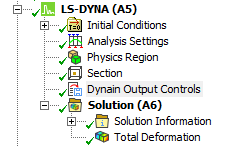
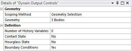
Some of the properties for the input cards can be customized using the Dynain Output Controls object. This includes the bodies that will be transferred, allowing the default of only flexible bodies to be overridden to all bodies or any subset. Beams are supported in this workflow. Other settings that can be controlled include the history variables that are transferred, contact and hourglass state at the end of the previous analysis, and time-independent boundary conditions (*BOUNDARY_SPC_NODE).
|
|
|
The other settings for these input file keywords take their default values. Refer to the LS-DYNA Keyword Manuals for details.
The Split Input File option allows you to save the different sections of the input file in separate files. An input.k file will be generated after solving and it will import the additional .k files generated by the Split Input File option. This is accomplished using the *INCLUDE command as seen in the following figure.
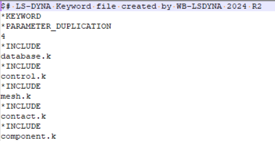
The input files generated are:
| database.k: keywords written to obtain output files containing results information |
| control.k: keywords written to define solution parameters and options |
| mesh.k: keywords written for the mesh |
| component.k: keywords written to define mesh components |
| contact.k: keywords written to define contacts between parts |
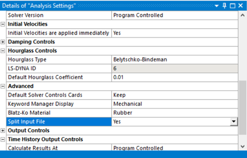
Enable this capability by setting the Split Input File option to Yes in the Advanced category of the Analysis Settings Details panel.
You must split the input file if you want to preserve the contact IDs between systems when using an LS-DYNA system in a downstream Workbench analysis. In order to get the transfer to work properly you must right click the Solution cell of the upstream system, select Properties and in the Properties pane select the Process Solution Data check box.