


After you have set up your case, and prior to solving it, you can check your case setup using the Case Check Dialog Box ( Figure 36.58: The Case Check Dialog Box). This function provides you with guidance and best practices when choosing case parameters and models. Your case will be checked for compliance in the mesh, models, boundary and cell zone conditions, material properties, and solver categories. Established rules will be available for each category, with recommended changes to your current settings. At your discretion, you may elect to apply the recommendations, or keep your current settings.
To access the Case Check Dialog Box (Figure 36.58: The Case Check Dialog Box), go to
![]() Solution → Run Calculation
Solution → Run Calculation ![]() Check
Case...
Check
Case...
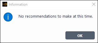
If there are no problems with your case setup, then an information dialog box (Figure 36.59: The Information Dialog Box) will appear stating that no recommendations need to be made at this time, otherwise, the Case Check Dialog Box will open.
In the Case Check dialog box, each of the tabs Mesh, Models, Boundaries and Cell Zones, Materials, and Solver may contain recommendations. For each of the tabs that are enabled, best practices will be listed.
In some cases, the dialog box will be split based on the method that the recommendation is applied. There are two ways you can apply the listed recommendations:
- Automatic Implementation
Ansys Fluent applies the change for you.
- Manual Implementation
You will manually change your case settings.
For additional information, see the following sections:
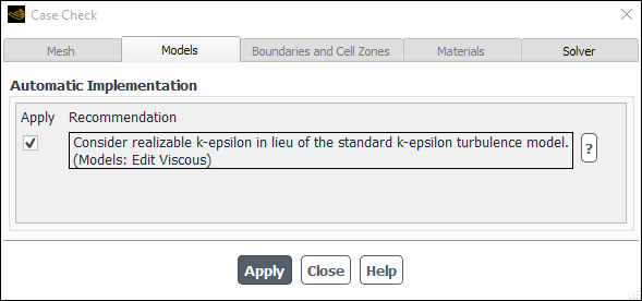
To the left of each of the recommendations listed under Automatic Implementation (for example, Figure 36.61: The Models Tab in the Case Check Dialog Box), there is an enabled Apply check box. An enabled check box will result in Ansys Fluent applying the change to your case automatically. If there are some recommendations that you do not want Ansys Fluent to implement automatically, then click the Apply check box to toggle off and disable the implementation of a particular recommendation. After going through all the tabs and determining which rules you want applied automatically, click the button at the bottom of the dialog box. Changes to your settings will be applied to all recommendations throughout the dialog box with an enabled Apply check box. Ansys Fluent will print a message in the console notifying you that the applied recommendation has been implemented.
Ansys Fluent will ask you if you want to save the case before proceeding to the next step. If you choose Yes, The Select File Dialog Box will open allowing you to save your case with the new settings. If you select No, all the changes made to the case file will be lost once you exit Ansys Fluent.
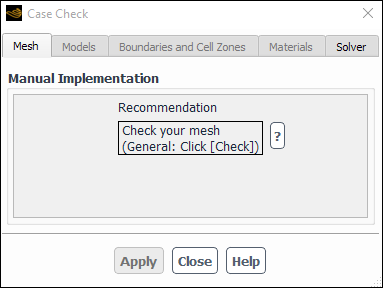
For recommendations that are listed under Manual Implementation, Ansys Fluent cannot apply the changes for you. Therefore, if you opt to make a change to your current settings, based on the listed recommendations, then you will need to manually make the changes by opening the affected dialog boxes or task pages and applying what was recommended.
To the right of the recommendations is a ?, which essentially acts as a help button, leading you to related documentation on the specific topic.
At the bottom of each recommendation, there is a path that will guide you to the dialog box or task page where you can make the changes. For example, in the Mesh tab, you will see the following recommendation:
 Check your mesh.
 (General: Click [Check])
To perform the action, highlight General in the tree, then click the button in the Mesh group box. You will see a path for each recommendation, in each of the tabs.
Each of the case check rules are described in the following sections:
The following recommendations appear under the Mesh tab (Figure 36.60: The Mesh Tab in the Case Check Dialog Box):
Check your mesh.
If you have not already checked your mesh, it is best practice that you do so immediately after reading in your mesh, or after any mesh modification. To check your mesh go to
 Setup →
  General →
Check
General →
CheckChecking the mesh will help you detect any mesh trouble before you get started with your problem setup. You can learn more about the information obtained when checking your mesh, by going to Checking the Mesh.
Minimum Orthogonal Quality is less than 0.01. Consider improving the mesh quality before proceeding with your simulation.
Check the quality of your mesh immediately after reading in your mesh, or after any mesh modification. The quality of the mesh plays a significant role in the accuracy and stability of the numerical computation. You can learn more about the quality of your mesh by going to Mesh Quality.
Setup → General → Report
QualityPreview zone motion and mesh motion before beginning the simulation.
After setting up your case using the Dynamic Mesh model, it is worth while to preview your mesh prior to running your simulation. You can preview Zone Motion by going to
Setup → Dynamic Mesh →  Dynamic Mesh → Display Zone Motion...
To preview the Mesh Motion, go to
Setup → Dynamic Mesh → Dynamic Mesh → Preview Mesh Motion...or
Solution → Run Calculation  Preview Mesh Motion...
or
Solution → Run Calculation →
Preview Mesh Motion...It is important that you preview zone motion first and then mesh motion. Zone motion shows the motion of all dynamic zones with the prescribed rigid body motion, using the graphics library. It is a very fast process and does not alter the mesh. Previewing the zone motion will show you if the motion is set up properly (for example zones moving in the wrong direction or rotating about the wrong center). It is much more difficult to detect these problems with mesh motion because small time steps are performed and no continuous animation is shown.
Mesh motion should always be done for dynamic mesh cases with prescribed motion. Mesh motion will only show the validity of the mesh during the simulation. Mesh deformation and dynamic zones without rigid body motion will be considered during a mesh motion preview.
Both the Mesh Motion and Zone Motion dialog boxes will have a Preview button that will allow you to view the mesh or zone motion prior to running your case. You can obtain more information on mesh motion and zone motion by going to Previewing the Dynamic Mesh.
Translate the mesh for axisymmetric geometry containing nodes below the x-axis.
If either Axisymmetric or Axisymmetric Swirl is specified in the General task page and there are mesh nodes that fall below the x-axis, then it is recommended that you translate the mesh. Nodes below the
 axis are forbidden for axisymmetric cases, since the axisymmetric cell volumes are created by rotating
the 2D cell volume about the
axis are forbidden for axisymmetric cases, since the axisymmetric cell volumes are created by rotating
the 2D cell volume about the  axis; therefore nodes below the
  axis would create negative volumes. To find out if there are any nodes that lie below the x-axis,
perform a mesh check (Checking the Mesh). For information on translating the mesh, see Translating the Mesh. To access the Mesh Translate dialog box, go to
axis would create negative volumes. To find out if there are any nodes that lie below the x-axis,
perform a mesh check (Checking the Mesh). For information on translating the mesh, see Translating the Mesh. To access the Mesh Translate dialog box, go to Domain → Mesh → Transform
→ Translate...
Domain → Mesh → Transform
→ Translate...
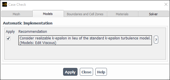
The following recommendations appear under the Models tab (Figure 36.61: The Models Tab in the Case Check Dialog Box):
Consider realizable k-epsilon in lieu of the standard k-epsilon turbulence model.
The realizable
 -
-  model is a more recent development of the standard
  -
-  model and differs from it in that the realizable
  -
-  model contains a new formulation for the turbulent viscosity, as well as a new transport equation
for the dissipation rate,
model contains a new formulation for the turbulent viscosity, as well as a new transport equation
for the dissipation rate,  , derived from an exact equation for the transport of the mean-square vorticity fluctuation.
realizable
 -
-  model means that the model satisfies certain mathematical constraints on the Reynolds stresses,
consistent with the physics of turbulent flows. For more information on the standard
model means that the model satisfies certain mathematical constraints on the Reynolds stresses,
consistent with the physics of turbulent flows. For more information on the standard  -
-  model and the realizable
  -
-  model, visit Standard k-ε Model and Realizable k-ε Model (in the Theory
Guide), respectively. Setup → Models →
model, visit Standard k-ε Model and Realizable k-ε Model (in the Theory
Guide), respectively. Setup → Models →  Viscous → Edit...
For information on all
 -
-  model options, go to Standard, RNG, and Realizable k-ε Models in the Theory Guide.
Disable DO/Energy coupling if the optical thickness is less than 10.
DO/Energy coupling should only be used when the optical thickness is greater than 10. Refer to Energy Coupling and the DO Model in the Theory Guide for more information.
Setup → Models → Radiation → Edit...Verify that the temperature specified for boundary zones that do not participate in the view factor calculation is appropriate.
When using the S2S radiation model, make sure that you set the temperature for boundaries that do not participate in the view factor calculation to an appropriate value. In most cases the appropriate value is the ambient temperature, which by default is assumed to be 300 K. See Specifying Boundary Zone Participation for more information.
Setup → Models → Radiation → Edit...Change the under-relaxation factor for the mixing plane model to 1.0.
If you have created a mixing plane, set the Under-Relaxation in the Mixing Plane dialog box to
1. Look under Global Parameters in Setting Up the Legacy Mixing Plane Model for information about the mixing plane under-relaxation. Domain → Mesh Models → Mixing
Planes...Enable the smoothing option for dynamic mesh simulations when remeshing.
When your case involves the use of dynamic meshes and remeshing is enabled, then it is recommended that you also perform smoothing on the mesh. For a complete discussion of smoothing and remeshing, see Setting Dynamic Mesh Modeling Parameters.
Setup → Dynamic Mesh → Dynamic MeshInclude turbulence interaction for the NOx model.
When running thermal NOx simulations and your flow is turbulent, then be sure to set the NOx Turbulence Interaction Mode.
Setup → Models → NOx → Edit...In turbulent combustion calculations, Ansys Fluent solves the density-weighted time-averaged Navier-Stokes equations for temperature, velocity, and species concentrations or mean mixture fraction and variance. Methods of modeling the mean turbulent reaction rate can be based on either moment methods or probability density function (PDF) techniques. Ansys Fluent uses the PDF approach.
To learn about how this feature is set up, go to Setting Turbulence Parameters.
Consider using the default Schnerr-Sauer or the Zwart-Gerber-Belamri cavitation model.
When using the mixture multiphase model with the Singhal et al. cavitation model enabled, consider changing it to either the Schnerr-Sauer or the Zwart-Gerber-Belamri cavitation model. Refer to Cavitation Models in the Theory Guide for more information.
Setup → Models → Phases
→ Interaction...
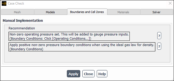
The following recommendations appear under the Boundaries and Cell Zones tab (Figure 36.62: The Boundaries and Cell Zones Tab in the Case Check Dialog Box):
Apply an axis boundary on the centerline (x-axis).
For geometry that is axisymmetric or axisymmetric swirl (as set in the General task page), the centerline (x-axis) boundary type should be set to axis. See Axis Boundary Conditions.
 Boundary Conditions
Change outlet boundary conditions. A combination of pressure and outflow boundaries is not compatible.
Outflow boundary conditions in Ansys Fluent are used to model flow exits where the details of the flow velocity and pressure are not known prior to solution of the flow problem. One of the limitations when using outflow boundary conditions is that outflow boundary conditions are not compatible with pressure inlets. Therefore, it is recommended that you use velocity or mass-flow inlets instead of pressure inlets when used in combination with outflow boundaries. See Outflow Boundary Conditions for a list of limitations that exist with outflow boundaries.
Setup → Boundary ConditionsChange outlet boundary conditions. Outflow boundary conditions are not compatible with the ideal gas law for density.
Outflow boundaries cannot be used if you are modeling unsteady flows with varying density, even if the flow is incompressible. See Outflow Boundary Conditions for more limitations that exist with outflow boundaries.
Setup → Boundary ConditionsNon-zero operating pressure set. This will be added to gauge pressure inputs.
For cases that have density specified as the ideal gas law, and the operating pressure is greater than zero, the operating pressure will be added to the gauge pressure to yield the absolute pressure. For more information, see Density Inputs for the Ideal Gas Law for Compressible Flows and Operating Pressure, Gauge Pressure, and Absolute Pressure.
Setup → Boundary Conditions →
Operating Conditions...Apply positive non-zero pressure boundary conditions when using the ideal gas law for density.
In compressible flows , isentropic relations for an ideal gas are applied to relate total pressure, static pressure, and velocity at a pressure inlet boundary. Your input of total pressure,
 , at the inlet and the static pressure,
  , in the adjacent fluid cell are related, as described in Equation 7–93 Equation 7–94 of Calculation Procedure at Pressure Inlet Boundaries. It is recommended that pressure boundary
conditions are not set to zero for compressible flows that use the ideal gas law. Setup → Boundary Conditions
, in the adjacent fluid cell are related, as described in Equation 7–93 Equation 7–94 of Calculation Procedure at Pressure Inlet Boundaries. It is recommended that pressure boundary
conditions are not set to zero for compressible flows that use the ideal gas law. Setup → Boundary ConditionsReview turbulence specifications at flow boundaries. Default values detected.
If your case setup has any of the turbulence models enabled, be sure to review the default parameters for K and Epsilon or K and Omega for the Turbulence Specification Method in the outlet and inlet boundary conditions. Ansys Fluent’s default parameters for the (Backflow) Turbulent Kinetic Energy, (Backflow) Turbulent Dissipation Rate, and (Backflow) Specific Dissipation Rate are
1. You can either adjust the values, or select a different Turbulence Specification Method. For general information turbulence parameters, see Determining Turbulence Parameters. Setup → Boundary ConditionsAssign non-zero layer thicknesses for wall boundaries with shell conduction.
When the Shell Conduction option is enabled in the Wall boundary condition dialog box, Ansys Fluent will compute heat conduction for the wall not only in the normal direction, but also in the planar directions. To enable such computations, you must specify a nonzero Thickness for each layer in the Shell Conduction Layers dialog box. See Shell Conduction for information on shell conduction in thin walls.
Setup → Boundary ConditionsAssign a value of 0 or 1 for VOF at the inlet or outlet boundary conditions.
When enabling the VOF model, the Volume Fraction in the inlet and outlet boundary conditions for each phase should be set either to
0or1. No intermediate values are permitted. For general information on boundary condition setup, see Defining Multiphase Cell Zone and Boundary Conditions. Setup → Boundary ConditionsChange the outlet boundary condition. Outflow boundary condition is not compatible with current multiphase settings.
You cannot assign an outflow boundary condition when using the mixture and Eulerian multiphase models. Note the limitations of this boundary condition in Outflow Boundary Conditions. Ansys Fluent can model the effects of open channel flow using the VOF formulation. In such a case, outflow boundary conditions can be used at the outlet of open channel flows, to model flow exits where the details of the flow velocity and pressure are not known prior to solving the flow problem. See Open Channel Flow in the Theory Guide, under the heading Outflow Boundary, for more information.
Setup → Boundary ConditionsReview wall motion. Stationary wall motion relative to adjacent cell zone detected.
In cases where the fluid zone motion type is specified as Moving Mesh or Moving Reference Frame, all wall zones should be set to Moving Wall in the Momentum tab in the Wall boundary conditions dialog box. The wall motion should be defined Relative to Adjacent Cell Zone. The exception to this is if the walls are stationary in the absolute frame. To define wall motion, see Inputs at Wall Boundaries.
Setup → Boundary ConditionsAssign non-zero velocities when specifying a moving fluid zone.
If selecting either Moving Mesh or Moving Reference Frame in the Fluid dialog box, be sure to set nonzero values for the rotational and translational velocities. Refer to Defining Zone Motion for user inputs.
Setup → Cell Zone ConditionsReview flow specifications at inlet boundaries. Default values detected.
For mass-flow-inlet and velocity-inlet boundary conditions, the default values in Ansys Fluent are
 and
and  , respectively. Review the settings and adjust accordingly. See Default Settings at Velocity Inlet Boundaries and Default Settings at Mass-Flow Inlet Boundaries for default parameters of
velocity inlets and mass-flow inlets, respectively. Setup → Boundary Conditions
, respectively. Review the settings and adjust accordingly. See Default Settings at Velocity Inlet Boundaries and Default Settings at Mass-Flow Inlet Boundaries for default parameters of
velocity inlets and mass-flow inlets, respectively. Setup → Boundary ConditionsDefine the porous zone when using the heat exchanger model.
Heat exchanger models always require the definition of the porous media zone on the primary side for the macro model and for both primary and auxiliary sides for the dual cell model. See Streamwise Pressure Drop in the Theory Guide for more information.
Setup → Cell Zone Conditions
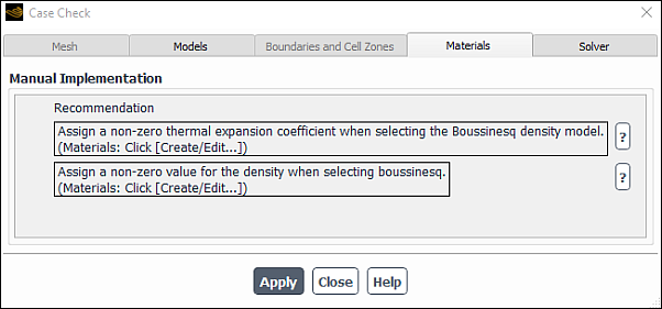
The following recommendations appear under the Materials tab (Figure 36.63: The Materials Tab in the Case Check Dialog Box):
Assign individual fluid Cps to polynomial functions of temperature.
For cases with species transport and volumetric reactions, it is best practice to specify the specific heat capacity
 as a polynomial that is a function of temperature. See Defining Properties for the Mixture and Its Constituent Species and Specific Heat Capacity as a Function of Temperature for information on defining material properties for the species in the
mixture. Setup → Materials
as a polynomial that is a function of temperature. See Defining Properties for the Mixture and Its Constituent Species and Specific Heat Capacity as a Function of Temperature for information on defining material properties for the species in the
mixture. Setup → MaterialsAssign a non-zero value for the density when selecting boussinesq.
The Boussinesq model is used for natural convection problems involving small changes in temperature. To enable the Boussinesq approximation for density, choose boussinesq from the Density drop-down list in the Create/Edit Materials dialog box and specify a constant value for Density. See Inputs for the Boussinesq Approximation.
Setup → MaterialsReview the absorption coefficient. Default value detected.
If any of the radiation models are enabled. Enter an absorption coefficient for the material listed (Radiation Properties).
Setup → MaterialsAssign a non-zero thermal expansion coefficient when selecting the Boussinesq density model.
When selecting boussinesq to describe the density of your material, be sure to enter a valid thermal expansion coefficient for your material. For detailed information on the Boussinesq model, see The Boussinesq Model.
Setup → Materials
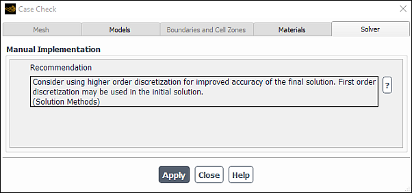
The following recommendations appear under the Solver tab (Figure 36.64: The Solver Tab in the Case Check Dialog Box):
Enable the unsteady solver option when selecting moving mesh for the fluid boundary.
If the motion type of the fluid boundary condition is specified as Moving Mesh, then your case should be specified as Transient in the General task page. Visit Setting Up the Sliding Mesh Problem for steps on setting up moving mesh problem.
Setup → GeneralAssign LSQ cell-based gradient reconstruction.
The least squares cell-based averaging scheme is known to be as accurate as the node-based gradient for irregular unstructured meshes, but less expensive to compute than the node-based gradient. Therefore, it is recommended that least squares cell-based gradient reconstruction is used. See Evaluation of Gradients and Derivatives in the Theory Guide for more information on gradient options.
Solution → MethodsChange the under-relaxation factor for the energy equation to at least 0.90.
You should set the energy under-relaxation factor between 0.90 and 1.0. If you decide to apply this recommendation, then Ansys Fluent will automatically set the energy under-relaxation factor to
0.90. If you want to increase this value, you can manually make the change by going to the Solution Controls task page. See Solution Strategies for Heat Transfer Modeling for the under-relaxation of the energy equation. Solution → ControlsIncrease the NOx under-relaxation factor to at least 0.90.
If the NOx model is enabled, set the NOx under-relaxation factor to a value of at least 0.90 to fully converge the solution. Note that the under-relaxation factor could be lower at the start of the run, but can then be increased after an initial solution is obtained. If you decide to apply this recommendation, then Ansys Fluent will automatically set the NOx under-relaxation factor to
0.90. If you want to increase this value, you can manually make the change by going to the Solution Controls task page. See Using the NOx Model. Solution → ControlsIncrease the Discrete Ordinates under-relaxation factor to at least 0.90.
If the Discrete Ordinates (DO) radiation model is enabled, set the radiation under-relaxation factor to a value of at least 0.90 to fully converge the solution. Note that the under-relaxation factor could be lower at the start of the run, but can then be increased after an initial solution is obtained. If you decide to apply this recommendation, then Ansys Fluent will automatically set the radiation under-relaxation factor to
0.90. If you want to increase this value, you can manually make the change by going to the Solution Controls task page. See DO Solution Parameters. Solution → ControlsIncrease the P1 under-relaxation factor to 1.0.
If the P1 radiation model is enabled, set the radiation under-relaxation factor to 1.0 to fully converge the solution. Note that the under-relaxation factor could be lower at the start of the run, but can then be increased after an initial solution is obtained. If you decide to apply this recommendation, then Ansys Fluent will automatically set the radiation under-relaxation factor to
1.0. See P-1 Model Solution Parameters. Solution → ControlsIncrease the species and energy under-relaxation factors to at least 0.90.
For a case with species transport and energy defined, set the species and energy under-relaxation factors to a value of at least 0.90. If you decide to apply this recommendation, then Ansys Fluent will automatically set the species and energy under-relaxation factors to
0.90. If you want to increase this value, you can manually make the change by going to the Solution Controls task page. See Solution Procedures for Chemical Mixing and Finite-Rate Chemistry. Solution → ControlsAssign a value of 1 for the under-relaxation factor for unsteady DPM with 1 DPM update per time step.
It is recommended that the DPM under-relaxation factor be set to 1 for unsteady DPM with 1 DPM update per time step.
Solution → ControlsIncrease the mean mixture fraction under-relaxation factor to at least 0.90.
If the non-premixed or partially premixed combustion models are enabled, then it is best to set the mean mixture under-relaxation factor to a value of at least 0.90 to ensure full convergence. If you decide to apply this recommendation, then Ansys Fluent will automatically set the mean mixture under-relaxation factor to
0.90. If you want to increase this value, you can manually make the change by going to the Solution Controls task page. See Solving the Flow Problem. Solution → ControlsConsider using higher order discretization for improved accuracy of the final solution. First-order discretization may be used in the initial solution.
It is generally advisable to obtain an initial solution using first-order accurate discretization, however, second order discretization is recommended for improved accuracy of the final solution. See Choosing the Spatial Discretization Scheme for more information on discretization schemes.
Solution → MethodsSelect the absolute reference frame for initializing cases when using the MRF model.
When using the MRF model, always use the absolute reference frame while initializing the solution. Select Absolute under Reference Frame in the Solution Initialization task page. If the Relative to Cell Zone option is selected, which is the default option, the initial flow field can contain discontinuities, which can cause convergence problems in the first few iterations. Refer to Initializing the Entire Flow Field Using Standard Initialization for more information.
Solution → Initialization
InitializeChoose PRESTO! for the pressure discretization scheme.
When using the VOF model, it is recommended that you use PRESTO! as the pressure discretization scheme. This scheme is recommended for flows with high swirl numbers, a high-Rayleigh-number natural convection, high-speed rotating flows, flows involving porous media, and flows in strongly curved domains. See Choosing the Pressure Interpolation Scheme for more information.
Solution → Methods