When the Green-Gauss theorem is used to compute the gradient of the scalar at the cell center , the following discrete form is written as

(23–30)

where is the value of at the cell face centroid, computed as shown in the sections below. The summation is over all the faces enclosing the cell.

By default, the face value, , in Equation 23–30 is taken from the arithmetic average of the values at the neighboring cell centers, that is,

(23–31)

Alternatively, can be computed by the arithmetic average of the nodal values on the face.

(23–32)

where is the number of nodes on the face.

The nodal values, in Equation 23–32, are constructed from the weighted average of the cell values surrounding the nodes, following the approach originally proposed by Holmes and Connel [255] and Rauch et al. [545]. This scheme reconstructs exact values of a linear function at a node from surrounding cell-centered values on arbitrary unstructured meshes by solving a constrained minimization problem, preserving a second-order spatial accuracy.

The node-based gradient is known to be more accurate than the cell-based gradient particularly on irregular (skewed and distorted) unstructured meshes, however, it is relatively more expensive to compute than the cell-based gradient scheme.

In the density-based solver, the stability of the node-based gradient can be reduced by the presence of tetrahedral elements along domain boundaries. To regain robustness on tetrahedral and mixed meshes, it is recommended to select the extended node-based boundary option, available under the text command:

solve/set/nb-gradient-boundary-option? yes yes

By default, the density-based solver uses an improved treatment of symmetry and periodic boundaries in the node-based reconstruction gradient. This treatment ensures that the gradient respects symmetry and periodic constraints at the discrete level, thus better matching results obtained on an untruncated domain. This treatment can be controlled with the text command:

solve/set/nb-gradient-improved-symmetry-periodic? yes/no

In this method the solution is assumed to vary linearly. In Figure 23.6: Cell Centroid Evaluation, the change in cell values between cell and along the vector from the centroid of cell to cell , can be expressed as

(23–33)

Figure 23.6: Cell Centroid Evaluation

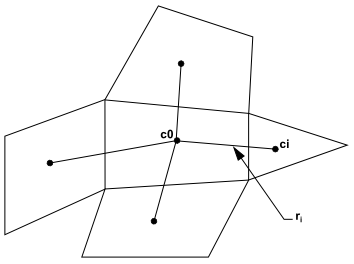
If we write similar equations for each cell surrounding the cell c0, we obtain the following system written in compact form:

(23–34)

Where [J] is the coefficient matrix that is purely a function of geometry.

The objective here is to determine the cell gradient () by solving the minimization problem for the system of the non-square coefficient matrix in a least-squares sense.

The above linear-system of equation is over-determined and can be solved by decomposing the coefficient matrix using the Gram-Schmidt process  [19]. This decomposition yields a matrix of weights for each cell. Thus for our cell-centered scheme this means that the three components of the weights () are produced for each of the faces of cell c0.

Therefore, the gradient at the cell center can then be computed by multiplying the weight factors by the difference vector ,

(23–35)

(23–36)

(23–37)

On irregular (skewed and distorted) unstructured meshes, the accuracy of the least-squares gradient method is comparable to that of the node-based gradient (and both are much more superior compared to the cell-based gradient). However, it is less expensive to compute the least-squares gradient than the node-based gradient. Therefore, it has been selected as the default gradient method in the Ansys Fluent solver.