


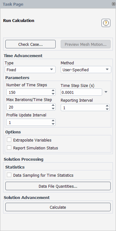
The Run Calculation task page allows you to start the solver iterations. See Performing Steady-State Calculations and Performing Time-Dependent Calculations for details about the items below.
Controls
- Check Case...
opens the Case Check Dialog Box.
- Preview Mesh Motion...
opens the Mesh Motion Dialog Box for transient simulations.
opens the Mesh Motion Dialog Box for steady simulations.
- Pseudo Time Settings
is available for fluid and solid zones when Global Time Step is selected from the Pseudo Time Method list in the Solution Methods Task Page as part of a steady-state case with the pressure-based coupled solver or density-based implicit solver. For details about the available options, see Pseudo Time Settings for the Calculation.
- Parameters
(for steady flow calculations) contains settings for running, reporting, and updating the calculation.
- Number of Iterations
sets the number of iterations to be performed.
- Reporting Interval
sets the number of iterations that will pass before residual monitors will be printed and plotted. The default is 1 (that is, reports will be updated after each iteration).
Note that the Reporting Interval also specifies how often Ansys Fluent should check if the solution is converged. For example, if your solution converges after 40 iterations, but your Reporting Interval is set to 50, Ansys Fluent will continue the calculation for an extra 10 iterations before checking for (and finding) convergence.
Important: The Reporting Interval only affects convergence checking of residuals, not of report definitions.
- Profile Update Interval
sets the number of iterations that will pass before user-defined functions for boundary profiles will be updated. This interval also controls the frequency at which named expression values will be updated.
- Time Advancement
(for transient flow calculations) contains settings related to time advancement.
- Type
allows you to specify the type of time stepping from the following selections. The type you select will determine what further selections are available in the Method drop-down list.
- Fixed
specifies that the time step size is fixed to a user-specified value or a value based on a specified period or frequency.
- Adaptive
specifies that the time step size changes during the solution, in order to either satisfy the Courant–Friedrichs–Lewy (CFL) condition, maintain a certain truncation error associated with the time integration scheme, or satisfy criteria that is specific for multiphase simulations.
- User-Defined Function
specifies that the time step size is defined by a user-defined function that uses the
DEFINE_DELTATmacro.
- Method
allows you to select one of the following, to specify how the time step size and number is determined:
- User-Specified
(for the Fixed type) specifies the use of a fixed time step size, equal to the specified Time Step Size.
- Period-Based
(for the Fixed type) allows you to specify a period (in seconds) as the basis for determining the time step size and number of time steps. See Inputs for Time-Dependent Problems for details.
- Frequency-Based
(for the Fixed type) allows you to specify a frequency (in hertz) as the basis for determining the time step size and number of time steps. See Inputs for Time-Dependent Problems for details.
- CFL-Based
(for the Adaptive type) specifies the use of a time step size that gets modified by Ansys Fluent as the calculation proceeds such that a version of the Courant–Friedrichs–Lewy (CFL) condition is satisfied, using the specified Courant Number. See CFL-Based Time Stepping for details.
- Error-Based
(for the Adaptive type) specifies the use of a time step size that gets modified by Ansys Fluent based on the specified truncation Error Tolerance. See Error-Based Time Stepping for details.
- Multiphase-Specific
(for the Adaptive type) specifies the use of a time step size that will be modified by Ansys Fluent based on the Global Courant Number in the interfacial cells. The time-step-size estimation based on the convective time scale is available for all multiphase models that use the implicit or explicit volume fraction formulation, with the exception of the wet steam model. For the VOF model, the time-step-size estimation includes additional constraints based on the physics and the moving mesh Courant number. See Multiphase-Specific Time Stepping for details.
- Duration Specification Method
(for the Adaptive or User-Defined Function type) specifies the way in which you will define the calculation duration. The duration can be defined by the total time, the total number of time steps, the incremental time, or the number of incremental time steps. In this context, "total" indicates that Fluent will consider the amount of time / steps that have already been solved and stop appropriately, whereas "incremental" indicates that the solution will proceed for a specified amount of time / steps regardless of what has previously been calculated.
- Parameters
(for transient flow calculations) contains settings for running, reporting, and updating the calculation.
- Number of Time Steps
sets or reports the number of time steps to be performed.
- Period
sets or reports the period to be used in the time step size calculation.
- Frequency
sets or reports the frequency to be used in the time step size calculation.
- Time Steps per Period
sets the number of time steps to divide each period into.
- Total Periods
sets the number of periods for the simulation to run.
- Total Time
sets the total time that will be calculated, including the time for which results were generated during previous calculations.
- Total Number of Time Steps
sets the total number of time steps to be performed, including the number of time steps performed in previous calculations.
- Incremental Time
sets the incremental time (that is, the additional time) for which results are to be calculated.
- Time Step Size
sets or reports the size of the (physical) time step
 .
.- Courant Number
allows you to specify the Courant number for CFL-based time stepping. The default value for the Courant number is 1.
- Error Tolerance
specifies the threshold value to which the computed truncation error is compared as part of error-based time stepping. Increasing this value will lead to an increase in the size of the time step and a reduction in the accuracy of the solution. Decreasing it will lead to a reduction in the size of the time step and an increase in the solution accuracy, although the calculation will require more computational time. For most cases, the default value of 0.01 is acceptable.
- Global Courant Number
allows you to specify the global Courant number for multiphase-specific time stepping. The default value for the Global Courant number is 2.
- User-Defined Time Step Size
contains a drop-down list of available user-defined functions (UDFs) that can be used to define the time step size.
- Number of Fixed Time Steps
specifies the number of fixed-size time steps that should be performed before the size of the time step starts to change. The size of the fixed time step is the value specified for Initial Time Step Size.
- Initial Time Step Size
is used for the first time step and then for as many subsequent steps as specified in the Number of Fixed Time Steps field. This value must fall between the minimum and maximum time step sizes. For a better startup, it should be chosen such that the Courant number initially remains close to 1 or your specified value (whichever is lower). Note that if you initialize the solution for a previously run case with adaptive time stepping, then Ansys Fluent will use the time step size saved in the case.
- Max Iterations/Time Step
(when using an implicit unsteady formulation) sets the maximum number of iterations to be performed per time step. If the convergence criteria are met before this number of iterations is performed, the solution will advance to the next time step. See Inputs for Time-Dependent Problems for details.
- Reporting Interval
sets the number of time steps that will pass before residual monitors will be printed and plotted. The default is 1 (that is, reports will be updated after each time step).
Note that the Reporting Interval also specifies how often Ansys Fluent should check if the solution is converged.
Important: The Reporting Interval only affects convergence checking of residuals, not of report definitions.
- Profile Update Interval
sets the number of iterations that will pass before user-defined functions for boundary profiles will be updated. This interval also controls the frequency at which named expression values will be updated.
- Time Step Size Update Interval
specifies the number of time steps that will pass before the time step size is updated for adaptive time stepping methods.
- Settings...
opens the Adaptive Time Stepping Dialog Box, so that you can define further settings for the adaptive time stepping method.
- Options (unsteady)
contains options related to unsteady calculations.
- Extrapolate Variables
instructs Ansys Fluent to predict the solution variable values for the next time step and then input that predicted value as an initial guess for the inner iterations of the current time step.
- Report Simulation Status
opens the Simulation Status Dialog Box, which reports details about the simulation.
- Specify Solid Time Step Size
enables a different time step size to be specified for solid zones, so that it is either user specified or automatically calculated. Using this option to specify a larger solid time step size reduces the risk of convergence issues. It is only available for transient cases, when there is a solid zone in the domain and energy is enabled. See Specifying the Solid Time Step Size for details.
When this option is enabled, the following are available in the Solid Time Stepping group box:
- Method
specifies how the time step size is determined for solid zones.
- Time Step Size
specifies the time step size for solid zones when you have selected User-Specified for the Method.
- Loosely Coupled Conjugate Heat Transfer
works in conjunction with the Specify Solid Time Step Size option (and thereby enables the use of a user-specified time step size for solid zones that can be larger than that used for the fluid zones) to increase the robustness of the energy equation calculation, and specifies that multi-domain architecture is used within a single Fluent session to enhance the performance of the simulation. It enables a loose coupling of the fluid and solid zone calculations, either at a specified time period or number of fluid time steps. For further details on using this option and its limitations, see Loosely Coupled Conjugate Heat Transfer.
When this option is enabled, the following are available in the Loosely Coupled Conjugate Heat Transfer group box for steady flows:
- Coupling Method
allows you to select from the following to determine how the coupling is performed.
- Instantaneous Implicit
specifies that the fluid-solid interface is solved in a fully coupled manner like conventional coupled thermal boundary condition at each coupling step. For details, see Thermal Conditions for Two-Sided Walls.
- Time-Averaged Explicit
specifies that Dirichlet – Neumann explicit thermal coupling is employed at each coupling step. A convective thermal boundary condition is applied at the wall adjacent to the solid and the instantaneous solid-side temperature is applied on the wall adjacent to the fluid. Time-averaged heat flow on the fluid side is used to compute the convective thermal boundary condition parameters (heat transfer coefficient and free-stream temperature) on the solid side.
- Coupling Controls
provides the following controls:
- Coupling Frequency Basis
specifies how you will define the coupling frequency. With the Instantaneous Implicit coupling method, you can select Time so that the coupling is performed at a set Time Period; otherwise (if you are not using adaptive time stepping), you can select Fluid Time Steps so that the coupling is performed at a set Number of Fluid Time Steps.
- Time Period
sets the time period for when solid calculations are solved and coupled with the fluid calculations. This field is available when Time is selected from the Coupling Frequency Basis drop-down list.
- Number of Fluid Time Steps
sets the number of fluid time steps used to trigger the solution of the solid calculations and coupling with the fluid calculations. This field is available when Fluid Time Steps is selected from the Coupling Frequency Basis drop-down list.
- Average Over (Time Steps)
displays the number of time steps used for computing time-averaged thermal variables. This is available when Time-Averaged Explicit is selected for the coupling method, and is shown for information only. The input for this field is automatically copied from the specified Number of Fluid Time Steps.
- Options (steady-state, pressure-based solver),
contains options for steady-state simulations that use the pressure-based solver.
- Loosely Coupled Conjugate Heat Transfer
is an option that can increase the robustness of the energy equation calculation, and specifies that multi-domain architecture is used within a single Fluent session to enhance the performance of the simulation. It enables a loose coupling of the fluid and solid zone calculations at a specified number of iterations. For further details on using this option and its limitations, see Loosely Coupled Conjugate Heat Transfer.
When this option is enabled, the following are available in the Loosely Coupled Conjugate Heat Transfer group box for steady flows:
- Coupling Method
allows you to select from the following to determine how the coupling is performed.
- Implicit
specifies that the fluid-solid interface is solved in a fully coupled manner like conventional coupled thermal boundary condition at each coupling iteration. For details, see Thermal Conditions for Two-Sided Walls.
- Explicit
specifies that Dirichlet – Neumann explicit thermal coupling is employed at each coupling iteration. A convective thermal boundary condition is applied at the wall adjacent to the solid and the instantaneous solid-side temperature is applied on the wall adjacent to the fluid. Iteration-averaged heat flow on the fluid side is used to compute the convective thermal boundary condition parameters (heat transfer coefficient and free-stream temperature) on the solid side.
- Coupling Controls
provides the following controls:
- Number of Iterations
sets the number of iterations used to trigger the solution of the solid calculations and coupling with the fluid calculations.
- Average Over (Iterations)
displays the number of iterations used for computing iteration-averaged thermal variables. This is available when Explicit is selected for the coupling method, and is shown for information only. The input for this field is automatically copied from the specified Number of Iterations.
- Options (steady-state, density-based solver)
contains options for steady-state simulations that use the density-based implicit solver.
- Solution Steering
allows you to set parameters that will help Ansys Fluent guide the calculations to a converged solution. This option is only available for steady-state simulations that use the density-based implicit solver. See Solution Steering for more information. When enabled, the following options are available:
- Flow Type
allows you to select the flow type that best describes the flow in the solution domain. Five choices are available: incompressible, subsonic, transonic, supersonic, and hypersonic.
- Use FMG Initialization
allows for full multigrid initialization.
- First- to Higher-Order Blending
allows you to reduce the desired solution accuracy by selecting a blending factor less than 100%. The default setting is 100%. See First- to Higher-Order Blending in the Theory Guide for more information. The blending factor will be grayed out if Second Order Upwind discretization for the Flow equations is not selected in the Solution Methods task page. The solution accuracy may be reduced (typical values are 75% or 50%) if it is not possible to obtain a converged solution with the maximum second-order accuracy (blending = 100%).
- More Settings...
opens the Solution Steering Dialog Box.
- Courant Number
is a non-adjustable field displaying the current CFL number, which allows you to view it during the calculation.
- Solution Processing
contains controls related to the processing of the calculations.
- Acoustic
contains controls for simulations that use the FW-H acoustics model.
- Time Step Size for Acoustic Data Export
determines the highest frequency that the acoustic analysis reproduces. This is available for the density-based solver when both the explicit formulation and explicit transient formulation are selected.
- Acoustic Sources FFT...
opens the Acoustic Sources FFT Dialog Box. This button is only available for three-dimensional transient simulations, when the Export Acoustic Source Data in ASD Format option is enabled in the Acoustics Model dialog box.
- Acoustic Signals...
opens the Acoustic Signals Dialog Box.
- Pollutants
contains controls for simulations that model pollutant formation.
- Postprocess Pollutants
results in the automatic postprocessing of pollutants during a transient simulation.
- Max Post Iterations/Time Step
sets the maximum number of postprocessing iterations to be performed per time step. This field is available when the Postprocess Pollutants option is enabled.
- PDF Transport Time Averaging
contains solution controls for steady-state simulations that use the composition PDF transport model with the Lagrangian method.
- Iterations in Average
specifies the number of iterations included in the PDF transport time averaging. For recommendations on how to use this setting, see Monitoring the Solution.
- Iteration Increment
specifies the rate at which the number of iterations included in the PDF transport time averaging will increase in each subsequent iteration. For recommendations on how to use this setting, see Monitoring the Solution.
- Statistics
contains controls for sampling statistics.
- Data Sampling for Steady Statistics
enables the sampling of data during a steady-state calculation. See Performing Steady-State Calculations and Postprocessing for Time-Dependent Problems for details.
- Data Sampling for Time Statistics
enables the sampling of data during an unsteady calculation. See Inputs for Time-Dependent Problems and Postprocessing for Time-Dependent Problems for details.
- Sampling Interval
allows you to specify how often data samples are accumulated for computation of mean and RMS values. For example, a sampling interval of 5 means that only every 5th result is added to the statistical sampling. This is for Data Sampling for Steady Statistics and Data Sampling for Time Statistics.
- Sampled Iterations
reports the number of iterations over which data has been sampled for the postprocessing of the mean and RMS values.
- Sampled Time
reports the time period over which data has been sampled for the postprocessing of the mean and RMS values.
- Sampling Options...
opens the Sampling Options Dialog Box for the Data Sampling for Steady Statistics or Data Sampling for Time Statistics.
- Data File Quantities...
opens the Data File Quantities Dialog Box. This button is only available when you are writing in the legacy format (that is,
.datfiles).
- Solution Advancement
contains buttons that advance the solution.
- Calculate
starts the calculations. While the calculation is in progress, a progress bar will appear at the bottom of the Fluent window. For steady-state simulations, clicking the button next to the progress bar will interrupt the calculation at the earliest safe stopping point after the current iteration; for transient simulations, buttons are available that allow you to stop the calculation at the end of the current iteration or time step. Alternatively, you can type Ctrl+c in the console; for transient simulations, a single instance will stop the calculation at the end of the current time step, whereas typing it twice will stop it at the end of the current iteration.
continues the calculations. This button is available when you have enabled the Automatically Initialize and Modify Case option in the Calculation Activities task page.
restarts the calculation from the beginning. This button is available when you have enabled the Automatically Initialize and Modify Case option in the Calculation Activities task page.
For additional information, see the following sections:
- 51.16.1. Case Check Dialog Box
- 51.16.2. Adaptive Time Stepping Dialog Box
- 51.16.3. Simulation Status Dialog Box
- 51.16.4. Solution Steering Dialog Box
- 51.16.5. Acoustic Sources FFT Dialog Box
- 51.16.6. Acoustic Signals Dialog Box
- 51.16.7. Sampling Options Dialog Box
- 51.16.8. Zone-Specific Sampling Options Dialog Box
This function provides you with guidance and best practices when choosing case parameters and models. Your case will be checked for compliance in the mesh, models, boundary and cell zone conditions, material properties, and solver categories. Established rules are available for each category, with recommended changes to your current settings. Information about each of the recommendations is available in Checking Your Case Setup.
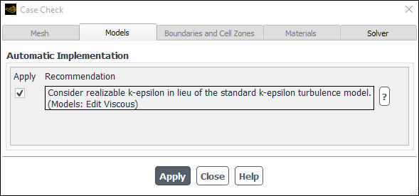
Controls
- Mesh
displays recommendations, if any, relating the to the mesh used in the case. See Checking the Mesh for details.
- Models
displays recommendations, if any, relating the to the models used in the case. See Checking Model Selections for details.
- Boundaries and Cell Zones
displays recommendations, if any, relating the to the cell zones or boundaries defined in the case. See Checking Boundary and Cell Zone Conditions for details.
- Materials
displays recommendations, if any, relating the to the materials defined in the case. See Checking Material Properties for details.
- Solver
displays recommendations, if any, relating the to the solver settings used in the case. See Checking the Solver Settings for details.
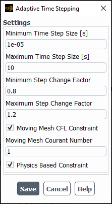
The Adaptive Time Stepping dialog box provides additional settings that affect the adaptive time stepping. This dialog box opens when you click Settings... in the Run Calculation task page. See Performing Time-Dependent Calculations for details about adaptive time stepping.
Controls
- Minimum/Maximum Time Step Size
specify the upper and lower limits for the size of the time step. If the time step size becomes very small, the computational expense may be too high; if the time step size becomes very large, the solution accuracy may not be acceptable to you. You can set the limits that are appropriate for your simulation.
- Minimum/Maximum Step Change Factor
limit the degree to which the time step size can change at each time step. Limiting the change results in a smoother calculation of the time step size, especially when high-frequency noise is present in the solution. For the CFL-Based and Multiphase-Specific methods, the time step size change factor is computed as the ratio between the current time step size and the previous time step size. For the Error-Based method, the time step size change factor is computed as the ratio between the specified truncation error tolerance and the computed truncation error.
- Moving Mesh CFL Constraint
(VOF model only) provides an option to include moving mesh CFL constraint in the time step size estimation. When this option is enabled, you can adjust Moving Mesh Courant Number, which has a default value of 1. For applications with a pure rigid body motion, Moving Mesh Courant Number may not be a significant parameter.
This item is available only for applications that involve either Frame Motion, or Mesh Motion, or Dynamic Mesh. See The Multiphase-Specific Time Stepping Algorithm for details.
- Physics Based Constraint
(VOF model only) provides an option to include physics-based constraints (depending on a specific type of physics involved, such as viscous, acoustic, gravitational, surface-tension-driven, and so on) in the time-step-size estimation. See The Multiphase-Specific Time Stepping Algorithm for details.
The Simulation Status dialog box reports details about the simulation.
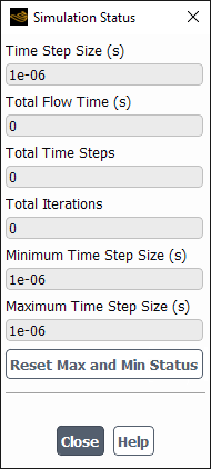
Controls
- Time Step Size
(for adaptive time stepping) reports the size of the last time step calculated for the simulation.
- Total Flow Time
reports the total time calculated for the simulation.
- Total Time Steps
reports the number of time steps calculated for the simulation.
- Total Iterations
reports the number of iterations calculated for the simulation.
- Minimum Time Step Size
(for adaptive time stepping) reports the size of the smallest time step used since either the start of the simulation or the last time you clicked the button in the Run Calculation task page, depending on whether you have clicked the button.
- Maximum Time Step Size
(for adaptive time stepping) reports the size of the largest time step used since either the start of the simulation or the last time you clicked the button in the Run Calculation task page, depending on whether you have clicked the button.
(for adaptive time stepping) resets the Minimum Time Step Size and Maximum Time Step Size fields, so that they consider only the values since the latest time you clicked the button in the Run Calculation task page.
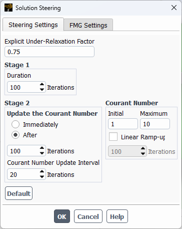
The Solution Steering dialog box is used to set the parameters that control the solution steering strategy. Solution steering will typically perform full multigrid (FMG) initialization followed by two iterative stages (Stage 1 and Stage 2). The purpose of Stage 1 is to navigate the solution from the difficult initial phase of the solution toward convergence by insuring maximum stability. During this stage, the solution is advanced gradually from 1st-order accuracy to maximum accuracy (user specified and typically 2nd-order) at a constant low CFL value. In Stage 2, the solution is driven hard towards convergence by regular adjustments of the CFL value to insure fast convergence as well as to prevent possible divergence. In Stage 2, the residual history is monitored and analyzed through regular intervals to determine if an increase or decrease in CFL value is needed to obtain fast convergence or to prevent divergence. See Solution Steering for details.
Controls
- Steering Settings
allows you to modify the steering parameters used in Stages 1 and 2.
- Stage 1
allows you to set parameters relating to stage 1.
- Duration
is the number of iterations in stage 1. The CFL number used during these iterations is set in the Initial field, in the Courant Number group box.
- Stage 2
allows you to set parameters relating to stage 2.
- Update the Courant Number
allows you to update the Courant number either Immediately, or After a specified number of iterations.
- Courant Number Update Interval
defines the frequency at which the Courant number is updated.
- Courant Number
allows you to set the starting (Initial) and maximum allowed (Maximum) Courant number values. The solution steering algorithm will not allow the solver to exceed the maximum Courant number, but will allow the solver to use a Courant number less than the initial Courant number if divergence in the solution has occurred.
- Explicit Under-Relaxation Factor
allows the solution to be under-relaxed to improve convergence.
- Default
resets any changes made to the parameters to their original default values.
- FMG Settings
allows you to set FMG parameters. For more information about FMG initialization, refer to Full Multigrid (FMG) Initialization.
- Number of Multigrid Levels
allows you to set the number of multigrid levels.
- Number of Cycles
allows you to set the number of cycles for a selected level.
- FMG Courant Number
allows you to set the FMG Courant number.
- Default
resets any changes to the original default values.
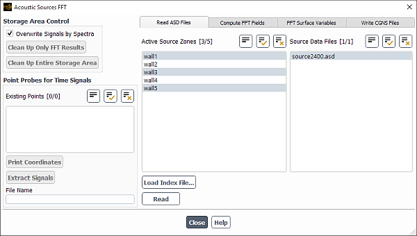
The Acoustic Sources FFT dialog box allows you to: read pressure signals from the acoustic source data (ASD) files (see Writing Source Data Files); compute Fourier spectra of these signals at the selected point probes and over the entire source zones; create surface variables for visualizing the spectral properties of the flow pressure signals; and write CGNS files of the spectrum data. See FFT of Acoustic Sources: Band Analysis and Export of Surface Pressure Spectra for details about the items below.
Controls
- Storage Area Control
allows you to specify how memory is allocated in the storage area (that is, the large memory array that stores the fields of the pressure histories and the computed fields of the Fourier spectra) when you compute the FFT fields in the Compute FFT Fields tab.
- Overwrite Signals by Spectra
specifies that the Fourier spectra displace in memory the original time signals, so that they are not kept after the FFT has been computed.
de-allocates the storage area—so that you can re-compute the FFT without re-reading the pressure histories—and deletes all variables created through the FFT Surface Variables tab. This button is only available when the Overwrite Signals by Spectra option is disabled.
de-allocates the storage area—so that you can re-read ASD files and re-compute the FFT with a clipped time range or different window function—and deletes all variables created through the FFT Surface Variables tab.
- Point Probes for Time Signals
allows you to get information about existing point probes and create pressure history files.
- Existing Points
lists all of the point probes created through the Point Surface Dialog Box that are available for selection.
prints in the console the coordinates of the point probe(s) selected in the Existing Points selection list.
creates ASCII files that contain the pressure histories of the point probe(s) selected in the Existing Points selection list.
- File Name
specifies a prefix for the names of the files created by the button.
- Read ASD Files
allows you to read pressure histories from the acoustic source data (ASD) files.
- Active Source Zones
is a list of the face zones for which you can read acoustic source data.
- Source Data Files
is a list of the ASD files you can read.
updates the Active Source Zones and Source Data Files lists by loading an ASCII index file.
reads the pressure signals from the selected items in the Active Source Zones and Source Data Files lists.
- Compute FFT Fields
allows you to compute FFT fields from the pressure signals read through the Read ASD Files tab.
- Sampling Data
allows you to reduce the time range of the signal data used to compute the FFT fields.
- Clip Time to Range
specifies that the time range of the data sampled is reduced to be between the Min and Max.
- Min
specifies the minimum value of the time range of the signal data when the Clip Time to Range option is enabled.
- Max
specifies the maximum value of the time range of the signal data when the Clip Time to Range option is enabled.
- Time Step
reports the size of the time step at which data was sampled.
updates the values that are displayed in the Spectral Resolution group box and that are used to compute the FFT fields, based on the settings in the Sampling Data group box.
- Spectral Resolution
displays the number of samples and the expected spectrum properties for the provided signals.
- Number of Samples
reports the total number of samples in the specified time range.
- Samples Used for FFT
reports the number of samples that will be used for FFT (see Table 40.2: Numbers of Data Points Supported by the Prime-Factor FFT Algorithm).
- Frequency Min & Step
reports the expected minimum frequency in the spectrum, which is also the expected frequency step.
- Frequency Max
reports the expected maximum frequency in the spectrum.
- Number of Modes
reports the expected number of Fourier modes in the spectrum.
- Window Function
specifies the shape of the window function used to enforce the signal's periodicity. See Windowing for details. The default is the Hanning window.
computes the FFT fields based on the settings in the Compute FFT Fields tab.
- FFT Surface Variables
allows you to create new Fluent variables for postprocessing using the spectrum fields computed through the Compute FFT Fields tab.
- Modes/Frequency Bands
specifies what the created variables will characterize.
- Octave Bands
specifies that the variables characterize proportional frequency bands corresponding to the standard technical octaves.
- 1/3 Octave Bands
specifies that the variables characterize proportional frequency bands corresponding to the standard technical thirds.
- Constant Width Bands
specifies that the variables characterize user-defined equidistant frequency bands.
- Set of Modes
specifies that the variables characterize the individual Fourier modes.
- Octave Central Frequencies
is a list of the octave central frequencies for which you can Fluent variables for postprocessing. This selection list is available when Octave Bands is selected from the Modes/Frequency Bands drop-down list.
- 1/3-Octave Central Frequencies
is a list of the 1/3-octave central frequencies for which you can Fluent variables for postprocessing. This selection list is available when 1/3-Octave Bands is selected from the Modes/Frequency Bands drop-down list.
- Frequency Min
specifies the minimum frequency of the set of modes for which you want to Fluent variables for postprocessing. This field is available when Set of Modes or Constant Width Bands is selected from the Modes/Frequency Bands drop-down list.
- Frequency Max
specifies the maximum frequency of the set of modes for which you want to Fluent variables for postprocessing. This field is available when Set of Modes or Constant Width Bands is selected from the Modes/Frequency Bands drop-down list.
- Number of Modes to Skip
allows you to thin or sample the modes for which you want to the Fluent variables for postprocessing. This field is available when Set of Modes is selected from the Modes/Frequency Bands drop-down list.
- Band Width
specifies the width of the constant width bands, for which you want to the Fluent variables for postprocessing. This field is available when Constant Width Bands is selected from the Modes/Frequency Bands drop-down list.
- Spectrum Property
displays the type of variables created according to the selected choice in the Modes/Frequency Bands drop-down list.
- PSD of dp/dt
is displayed when frequency bands are selected from the Modes/Frequency Bands drop-down list, in order to indicate that the created variables will be the power spectral density (PSD) fields, calculated for the time derivative of flow pressure.
- Surface Pressure Level
is displayed when frequency band is selected from the Modes/Frequency Bands drop-down list, in order to indicate that the created variables will be the surface pressure level (SPL) fields, in decibels.
- Real and Imaginary Amplitude Parts
is displayed when Set of Modes is selected from the Modes/Frequency Bands drop-down list, in order to indicate that the created variables will be the real and imaginary parts of the complex Fourier amplitudes, with a pair of variables per specified mode.
- Existing Variables
lists the processed variables that have been created by the button, and allows you to make selections for deletion using the button.
deletes the processed variables selected in the Existing Variables list from the storage area (as described previously), so that you can analyze more than the maximum of 20 individual modes or constant width bands that are allowed to exist at any one time.
When selected, and upon clicking Create, Fluent writes the area-averaged pressure data to an ASCII file in the XY plot file format.
When selected, and upon clicking Create, Fluent plots the area-averaged pressure data in the form of a bar chart in the graphics window.
creates new Fluent variables for postprocessing (based on your settings in the FFT Surface Variables tab), updates the Existing Variables selection list, and (when Set of Modes or Constant Width Bands is selected from the Modes/Frequency Bands drop-down list) prints information in the console.
- Write CGNS Files
allows you to write CGNS files of the spectrum data.
- Processed Source Zones
is a list of the zones you can export.
- Frequency Series
allows you to reduce the exported spectrum data.
- Reduce Frequency Series
specifies that the exported spectrum data is reduced to be between the Min and Max.
- Min
specifies the minimum of the frequency range to be exported when the Reduce Frequency Series option is enabled.
- Max
specifies the maximum of the frequency range to be exported when the Reduce Frequency Series option is enabled.
- Number of Frequencies to Skip
allows you to thin or sample the frequencies to be exported.
- Number of Frequencies per File
specifies the number of frequencies exported in each file. A value should be chosen based on the Number of Modes field of the Compute FFT Fields tab, in order to avoid creating either extremely large output files or a large number of very small files.
- File Name
specifies the base file name of the output files.
writes CGNS files of the spectrum data.
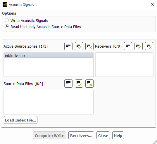
The Acoustic Signals dialog box is used to compute and save the sound pressure signals. See Postprocessing the FW-H Acoustics Model Data for details about the items below.
Controls
- Options
contains the options available for acoustic signal postprocessing.
- Write Acoustic Signals
enables the parameters needed to write the sound pressure data to files.
- Read Unsteady Acoustic Source Data Files
enables the parameters needed to compute the sound pressure signals using the source data saved to files.
- Active Source Zones
contains source zones you want to include to compute sound. See Specifying Source Surfaces for details.
- Receivers
contains all the receivers for which you can compute sound.
- Source Data Files
contains all the source data files that you can use to compute sound.
- Load Index File...
opens the Select File dialog box, in which you can select the index file for your computation.
- Write
writes the sound pressure data. This button will appear only when Write Acoustic Signals is selected under Options.
- Compute/Write
computes and saves the sound pressure data. This button will appear only when Read Unsteady Acoustic Source Data Files is selected under Options.
- Receivers...(button)
opens the Acoustic Receivers Dialog Box in which you can define additional receivers.
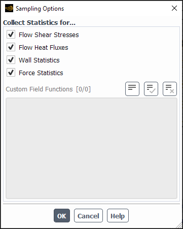
The Sampling Options dialog box allows you to specify a collection of statistics for: Flow Shear Stresses, Flow Heat Fluxes, Wall Statistics, DPM Variables, and Custom Field Functions.
Controls
- Collect Statistics for...
contains options for the variables you want to be able to postprocess.
- Flow Shear Stresses
allows you to enable or disable the flow shear stress statistics for postprocessing.
- Flow Heat Fluxes
allows you to enable or disable the flow heat fluxes statistics for postprocessing.
- Wall Statistics
allows you to enable or disable the wall statistics for postprocessing.
- Force Statistics
allows you to enable or disable the force statistics for postprocessing using cumulative plots (Cumulative Force, Moment, and Coefficients Plots).
- DPM Variables
allows you to enable or disable DPM variable statistics for postprocessing.
- Custom Field Functions
allows you to select the previously defined custom field functions you want to be able to postprocess.
The Zone-Specific Sampling Options dialog box allows you to specify which statistics are collected and where they are collected. Refer to Inputs for Time-Dependent Problems and Data Sampling for Steady Statistics for additional information.
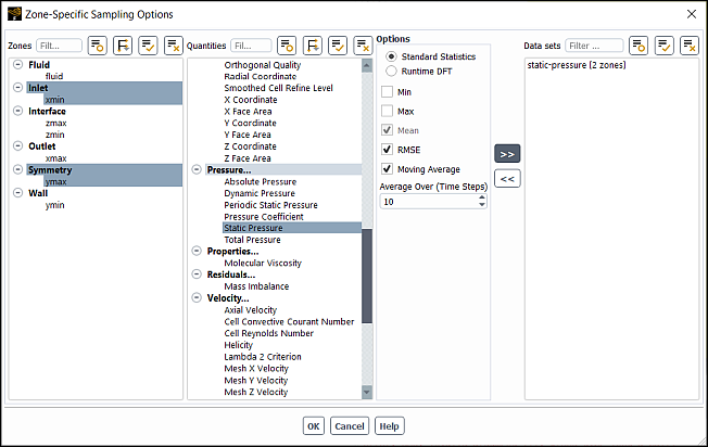
Controls
- Zones
lists the available locations where statistics can be collected.
- Quantities
allows you to specify which statistics are collected on the selected zone(s).
- Min
allows you to specify that the minimum value of the selected quantity(s) will be collected.
- Max
allows you to specify that the maximum value of the selected quantity(s) will be collected.
- Mean
shows that the average value of the selected quantity(s) will be computed and collected (this option is always enabled).
- RMSE
allows you to specify that the root mean square error of the selected quantity(s) will be computed and collected.
- Moving Average
allows you to specify an interval for averaging of the computed statistics.
- Average Over
specifies the number of iterations (steady simulations) or time steps (transient simulations) that will be used for computing the moving average.
Important: If you want to change the Average Over value for a dataset, you must remove it from the Data sets list (
 ) and re-add the same zones and quantities with the new
Average Over value.
) and re-add the same zones and quantities with the new
Average Over value.
- Runtime DFT
allows you to specify that the runtime discrete Fourier transform of the selected quantity(s) will be computed and collected.
- Add
clicking
 allows you to specify which statistics are collected on the selected
zone(s).
allows you to specify which statistics are collected on the selected
zone(s).- Remove
clicking
removes the selected Data Sets.